Racial inequality begins in early childhood
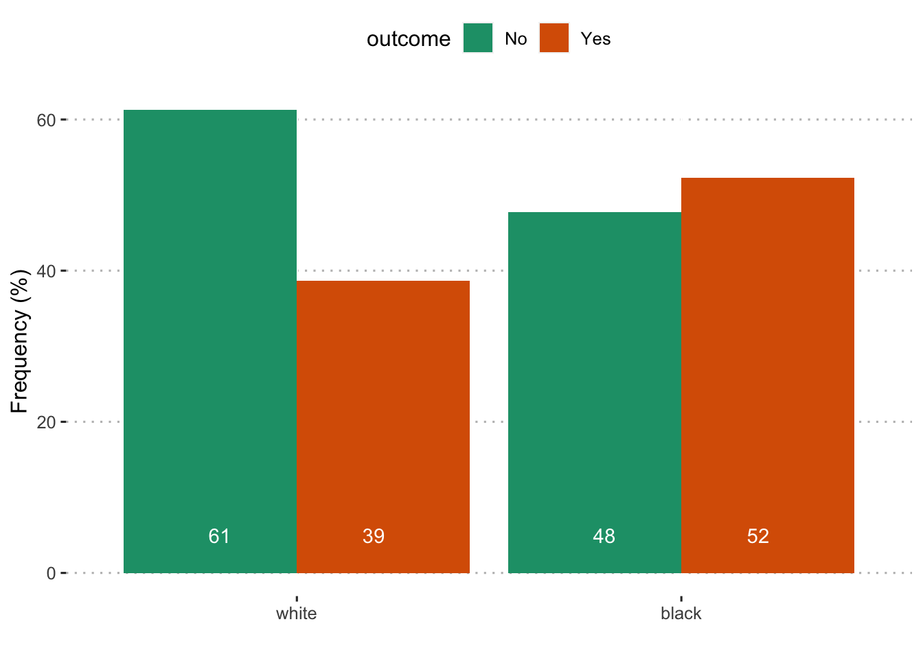
Responses ARE NOT WEIGHTED by race.
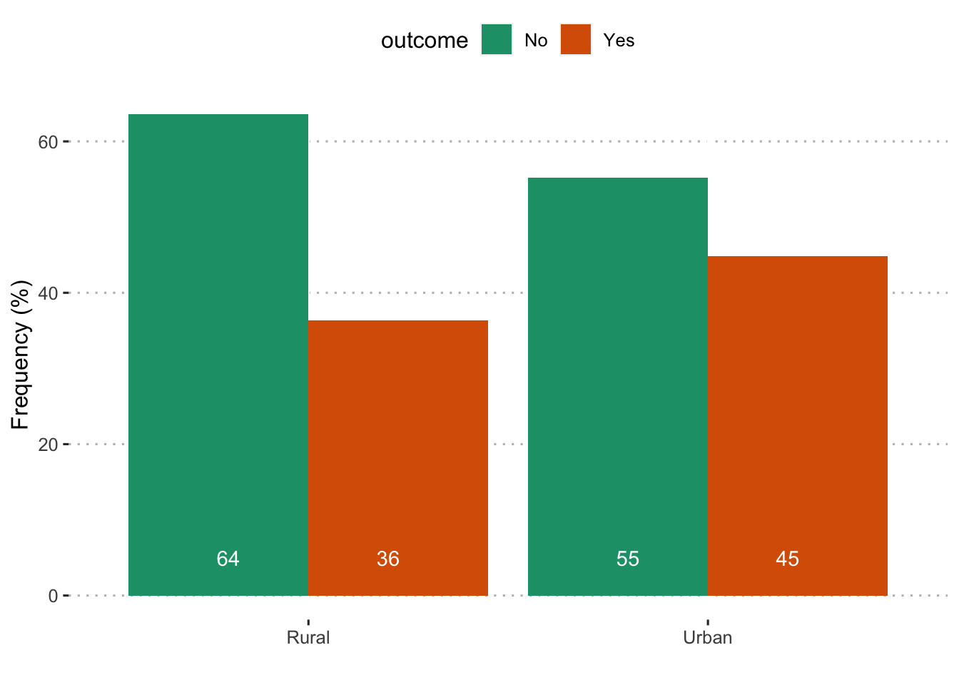
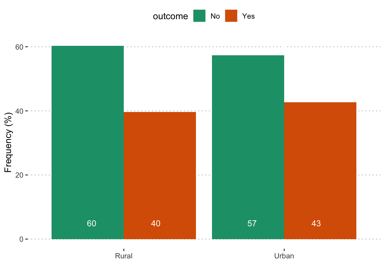
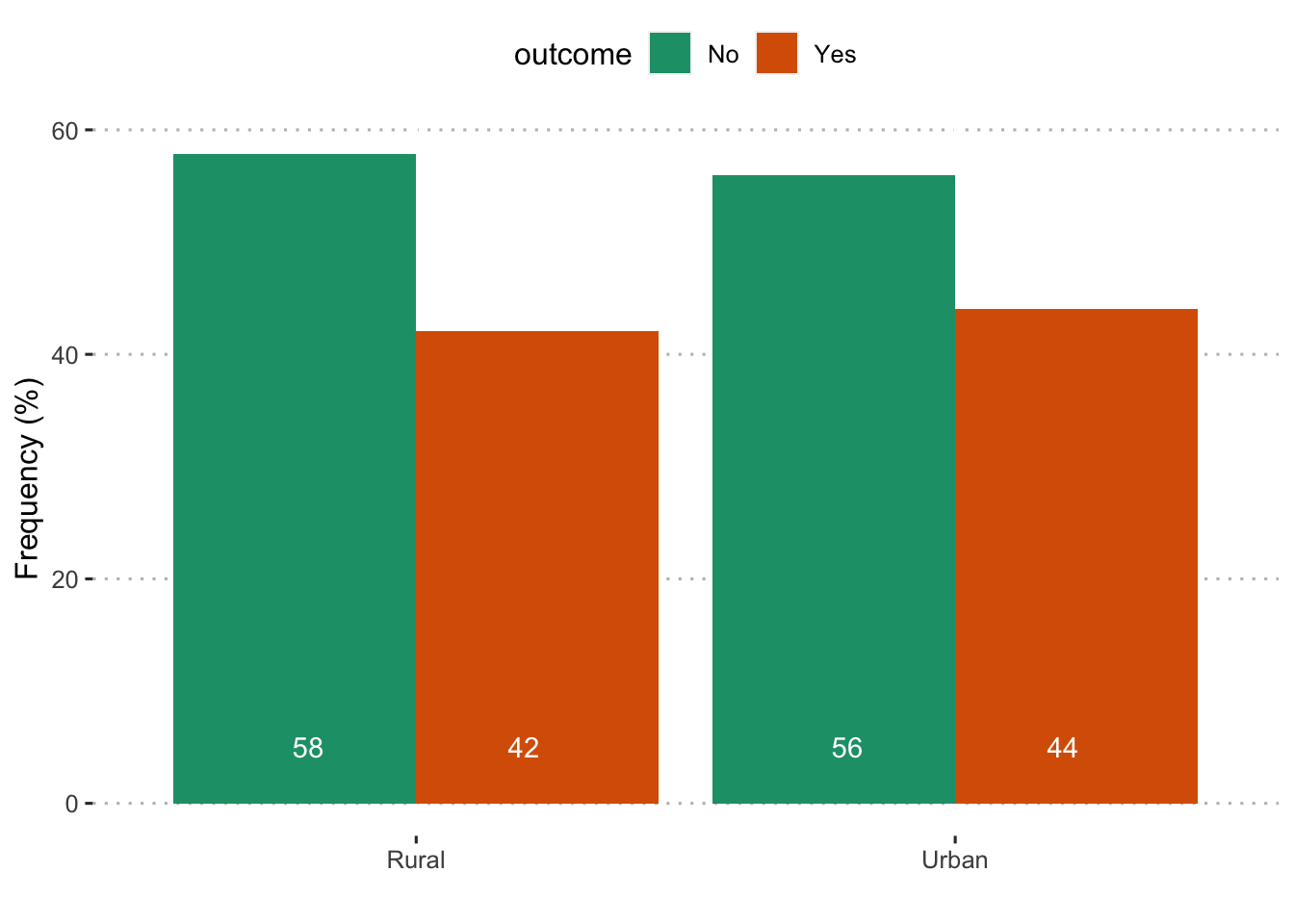
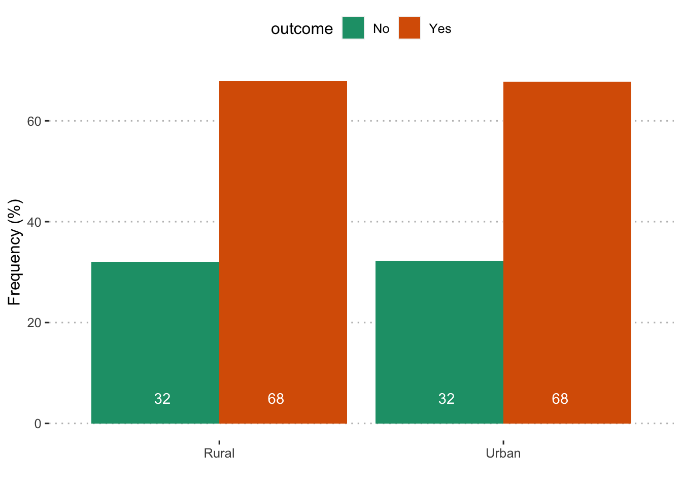
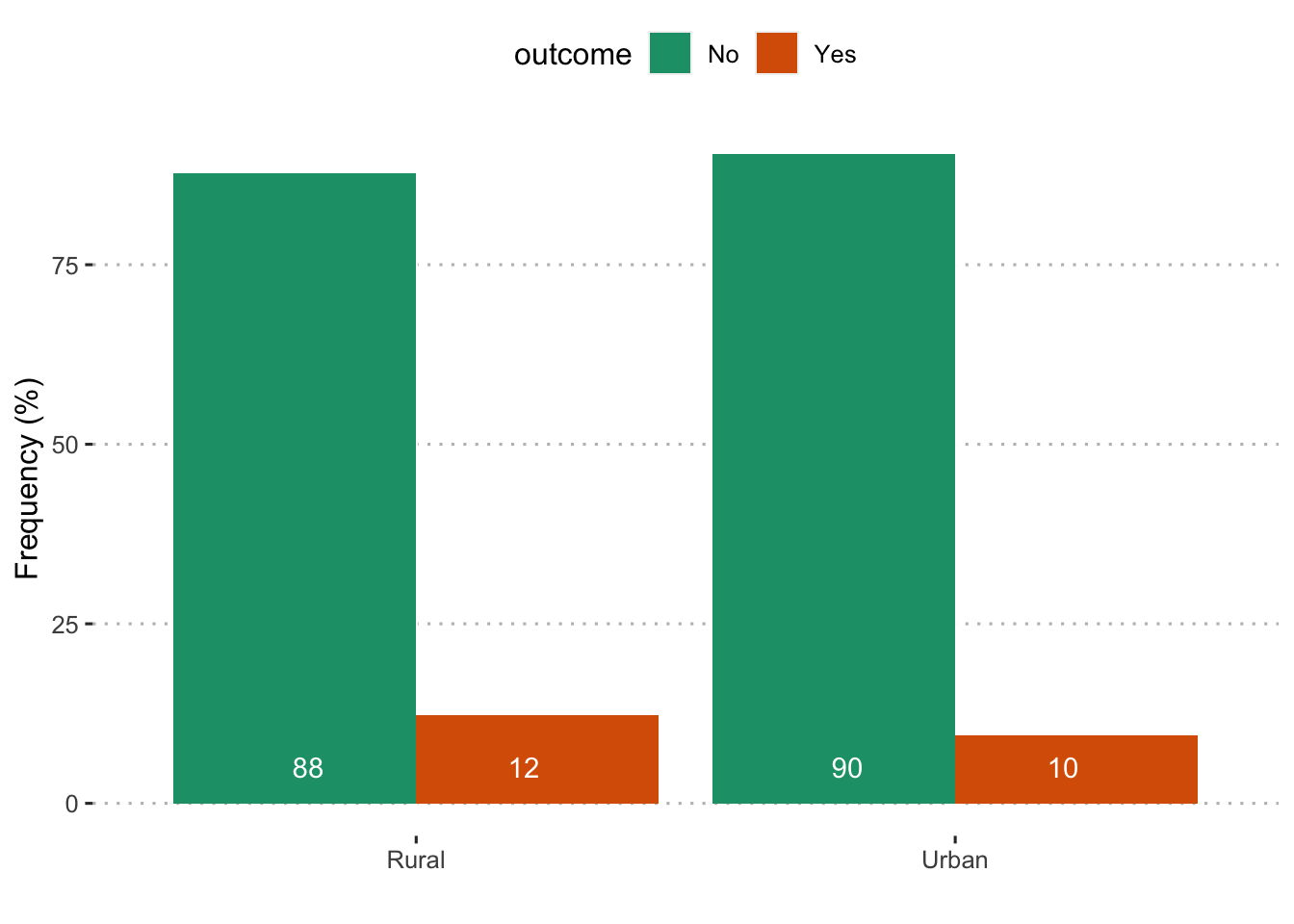
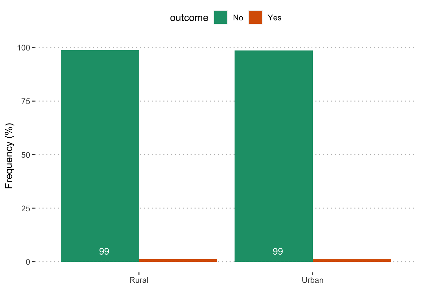
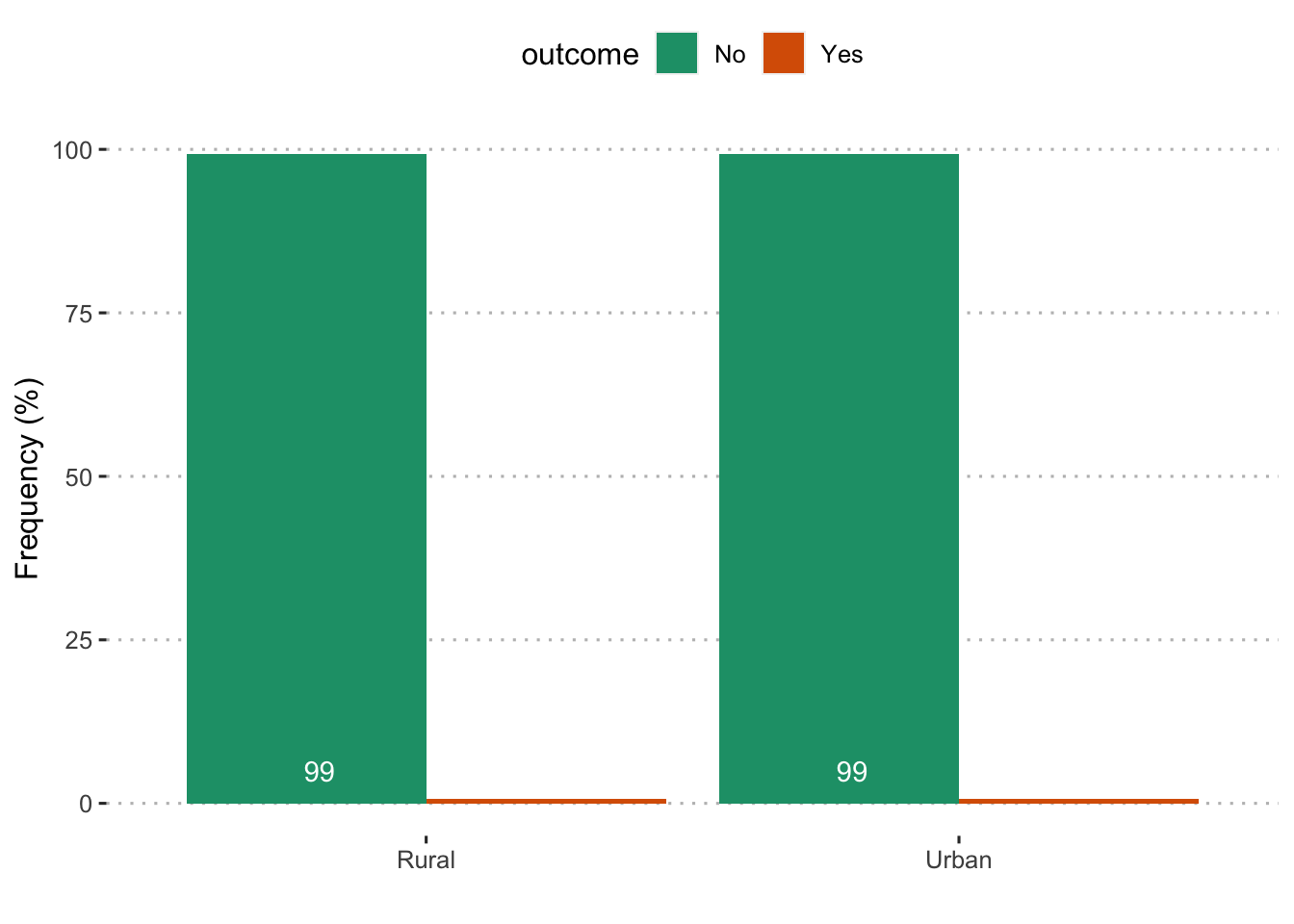
Rural communities are defined as zipcodes with density smaller than 500 people per square mile. Urban areas are zipcodes with density greater than 1000 people per square mile. Zipcodes between these two extremes are omitted.
Sample sizes
| Comparison | Group 1 | Group 2 |
|---|---|---|
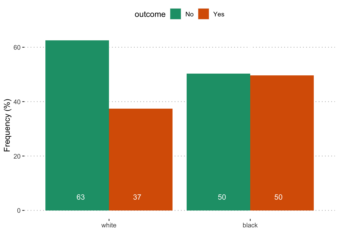
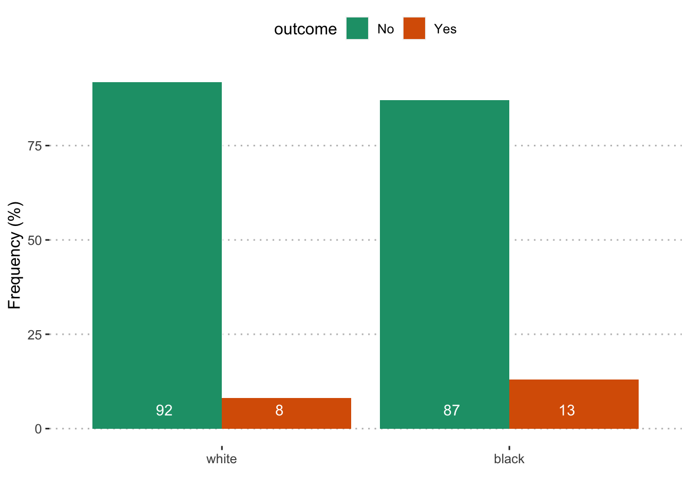
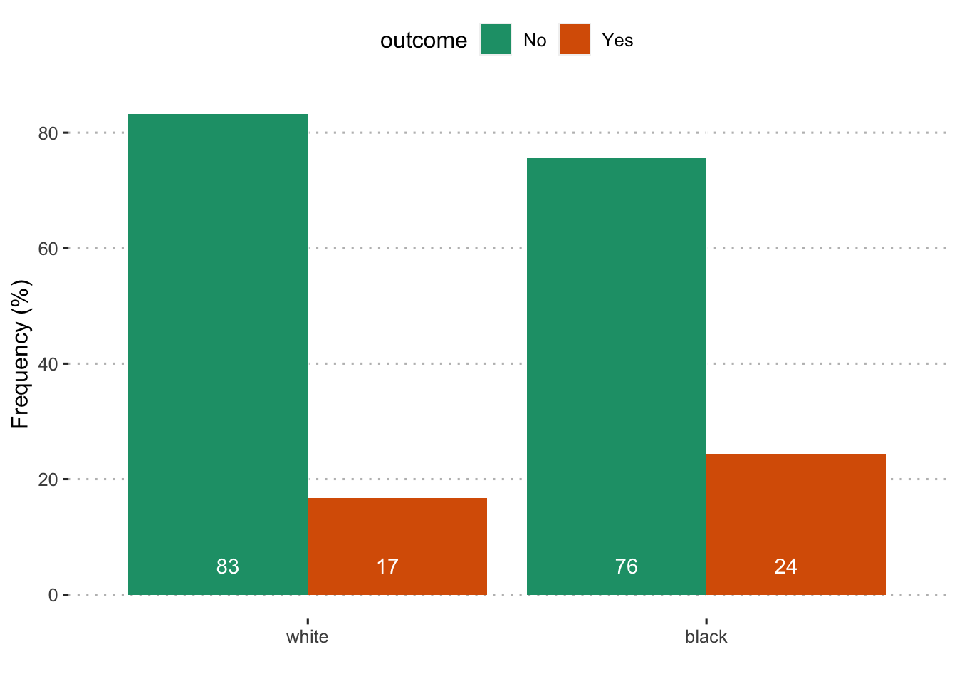
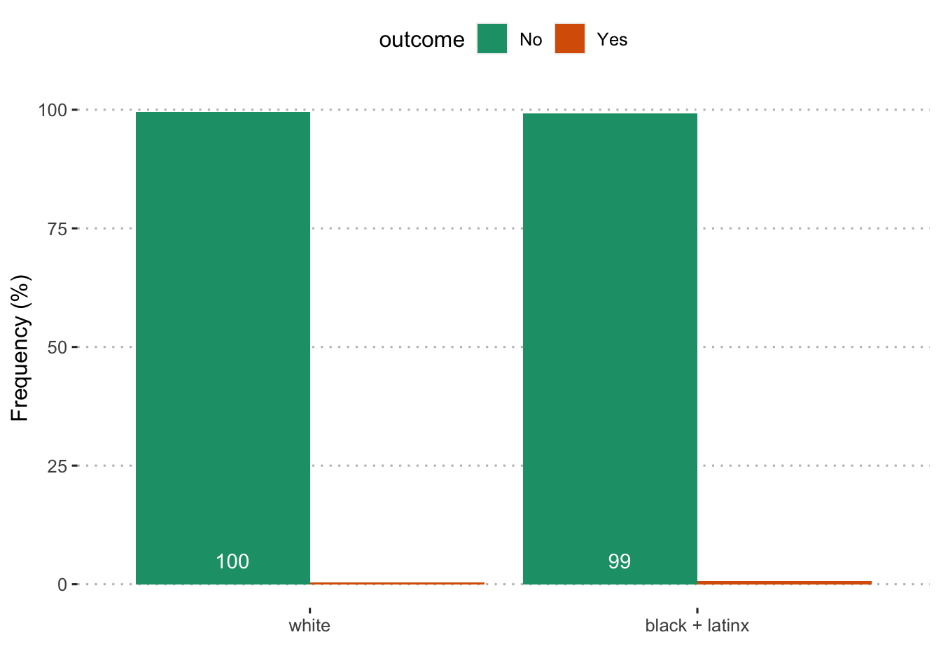
| 1 | Black | White |
| 771 | 6541 | |
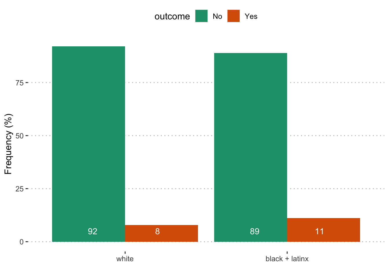
| 2 | Black + LatinX | White |
| 2186 | 5797 | |
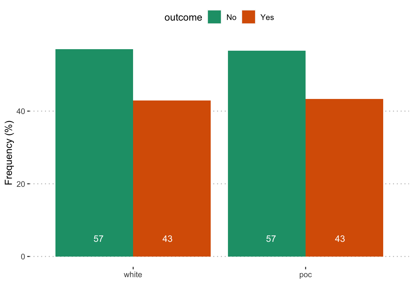
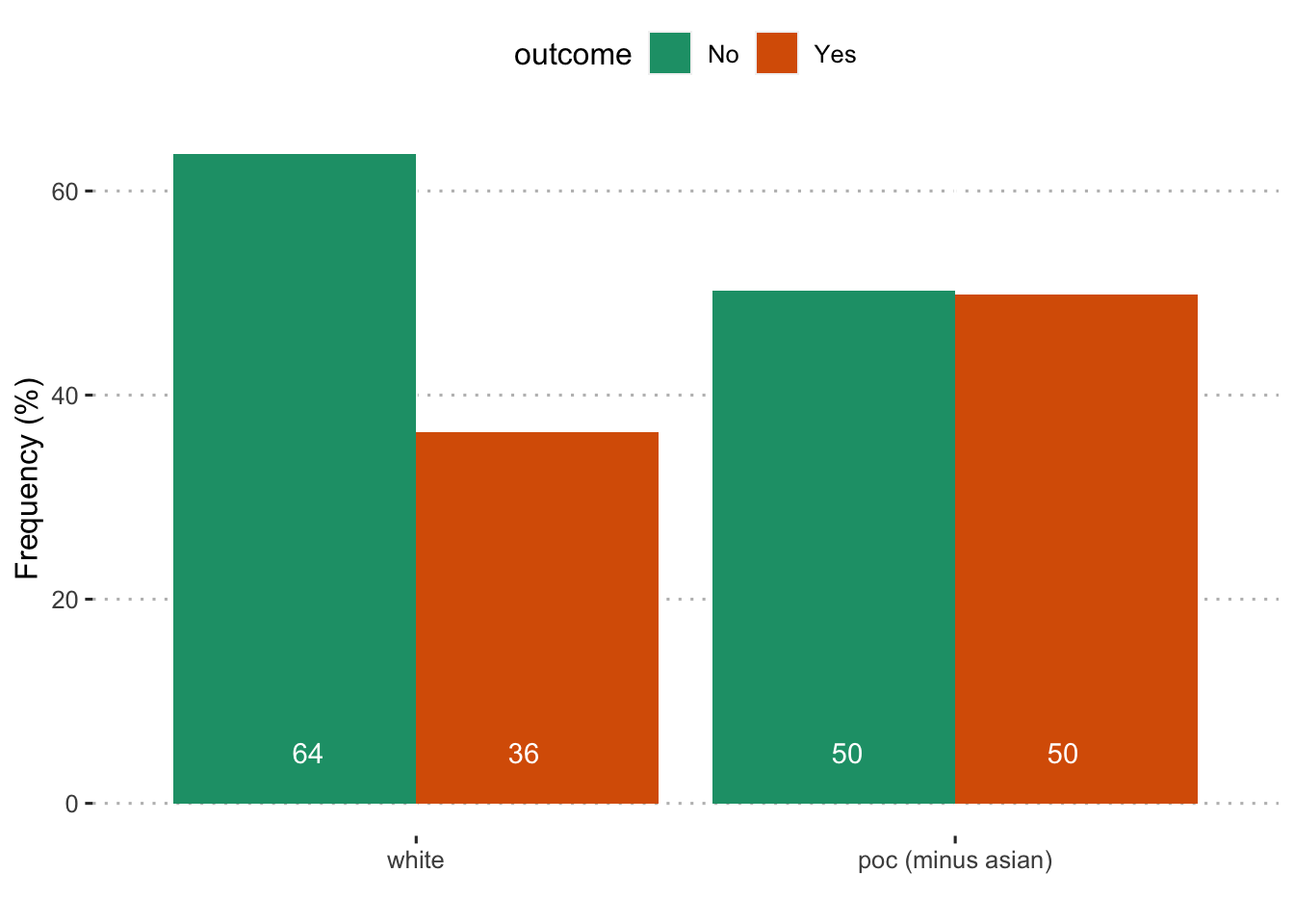
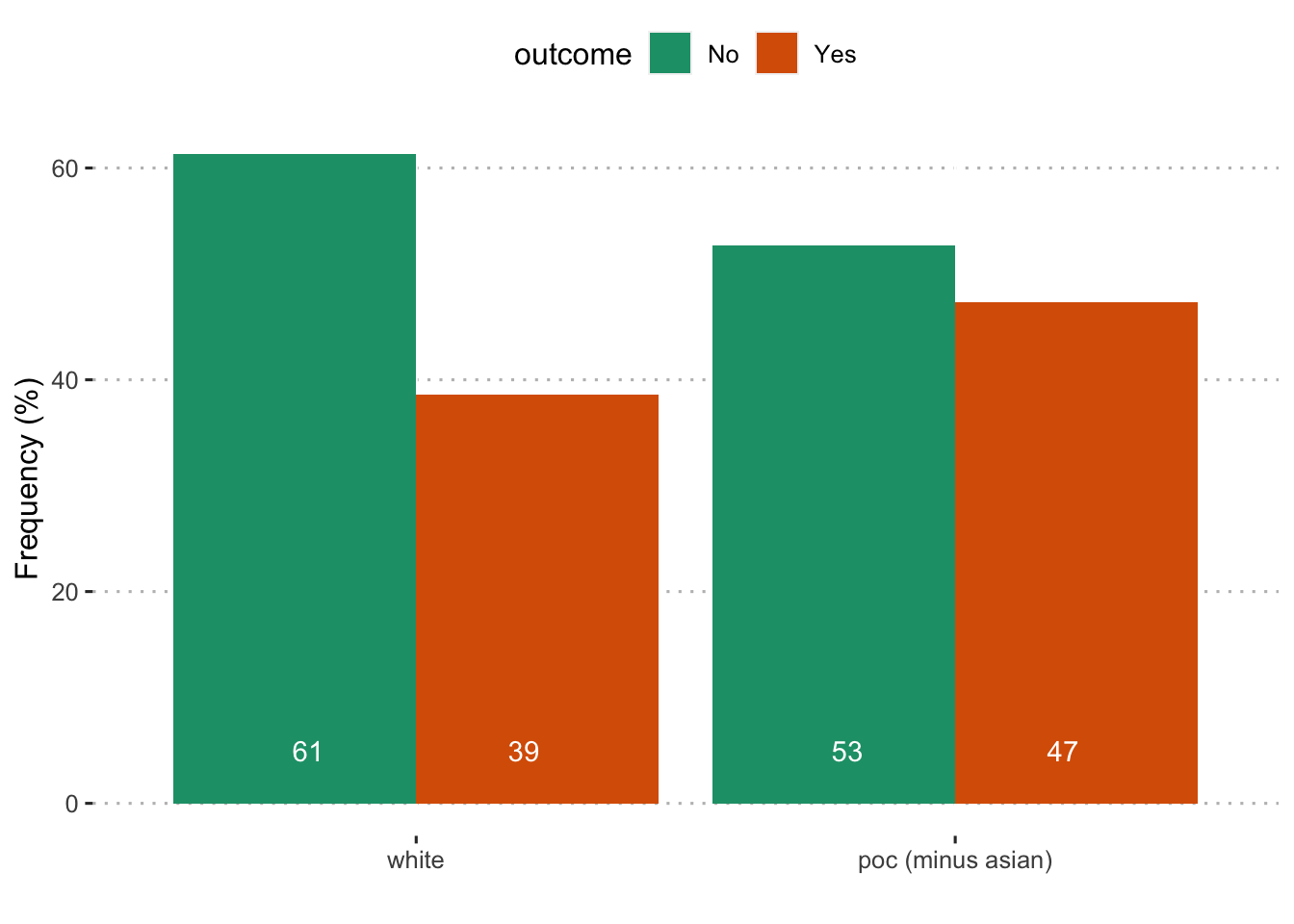
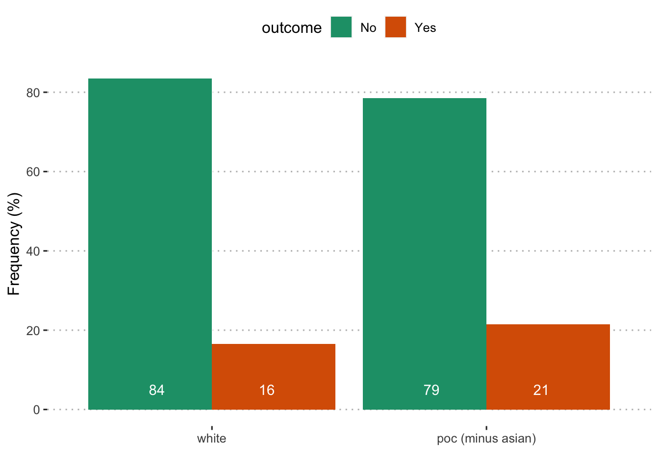
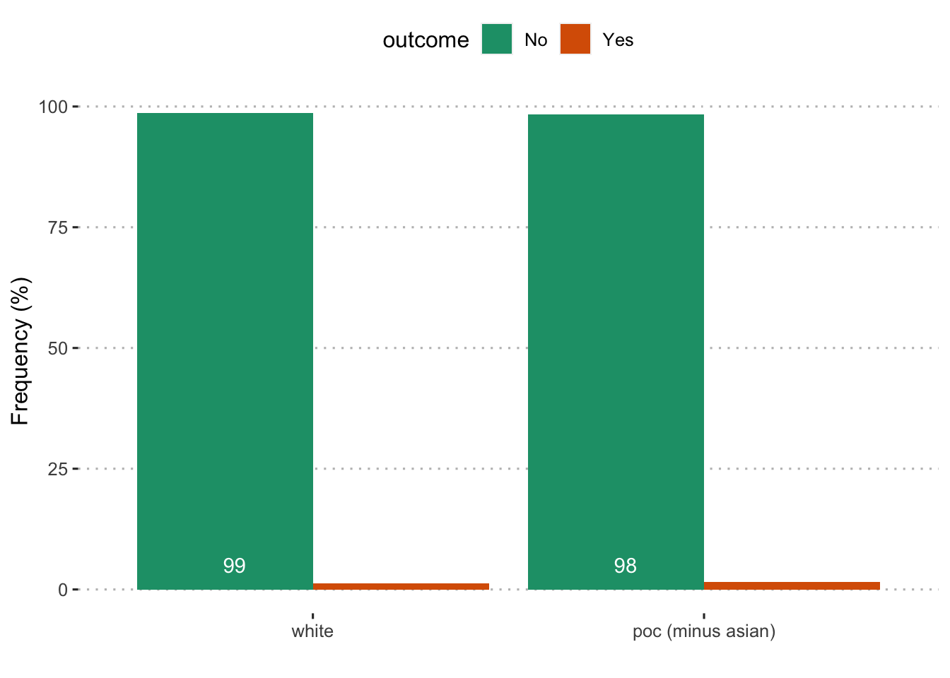
| 3 | POC (minus Asian) | White |
| 2554 | 5797 | |
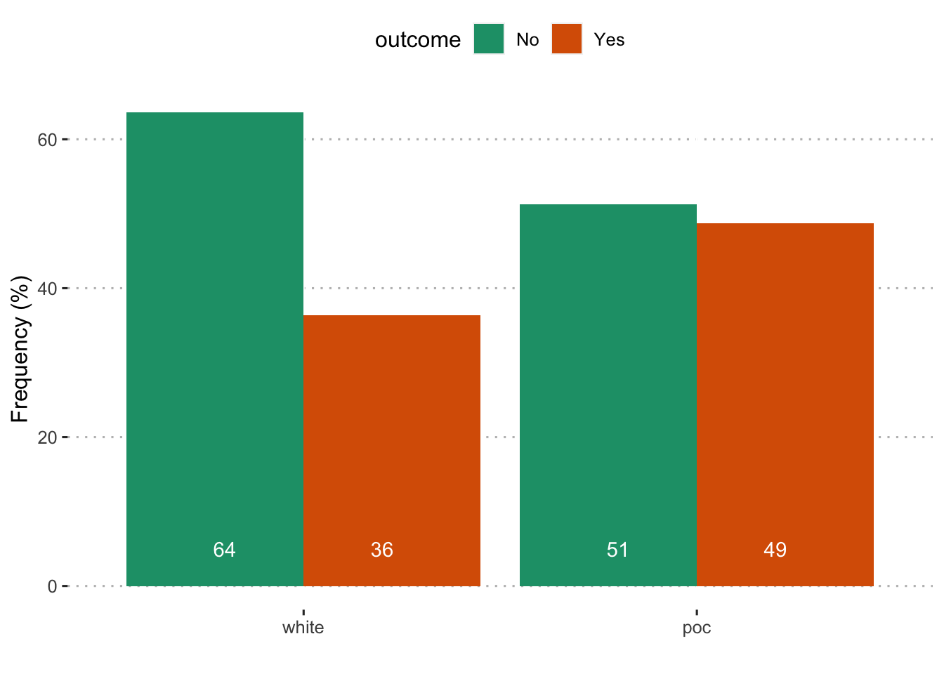
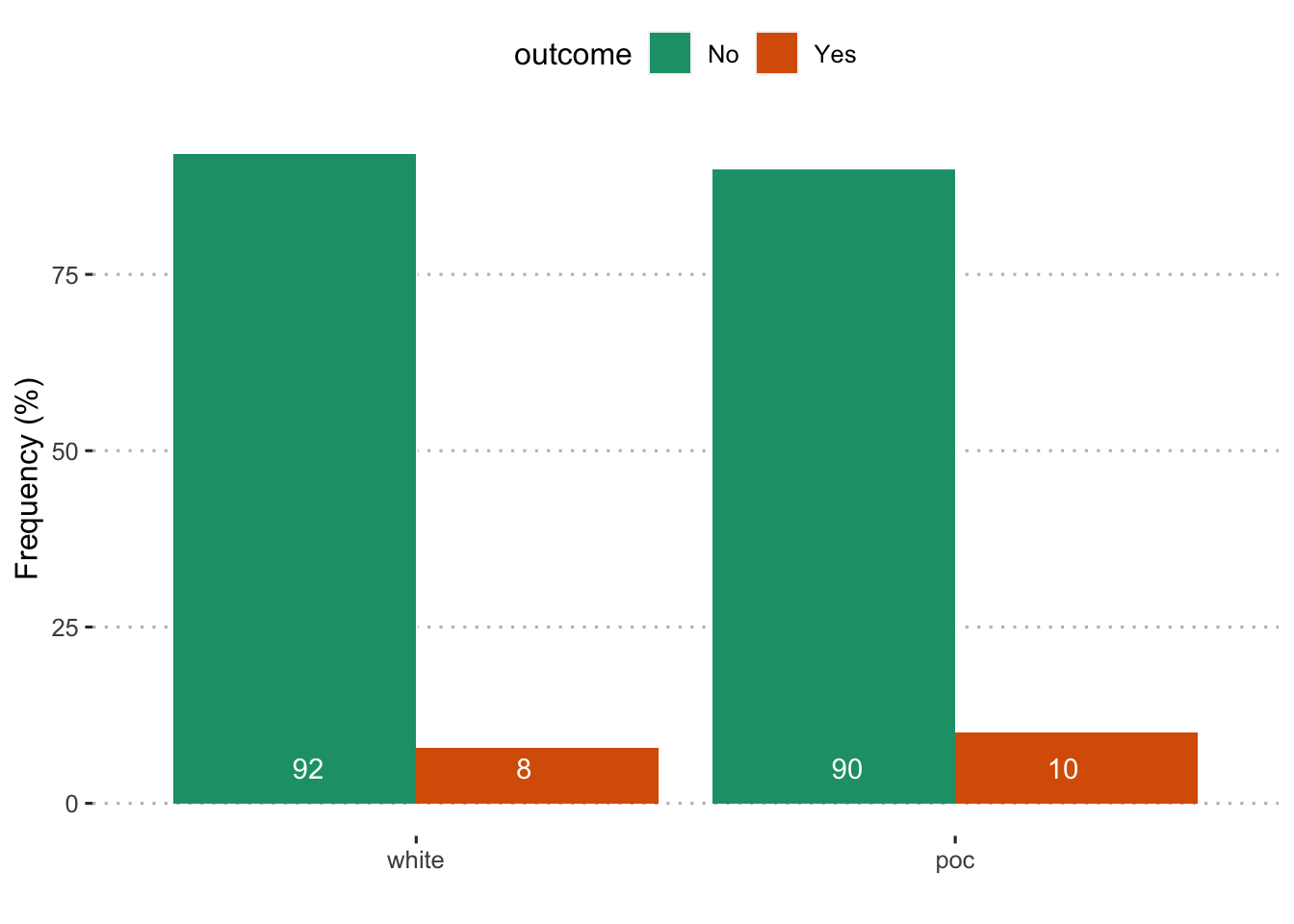
| 4 | POC | White |
| 2875 | 5797 |
Well-being
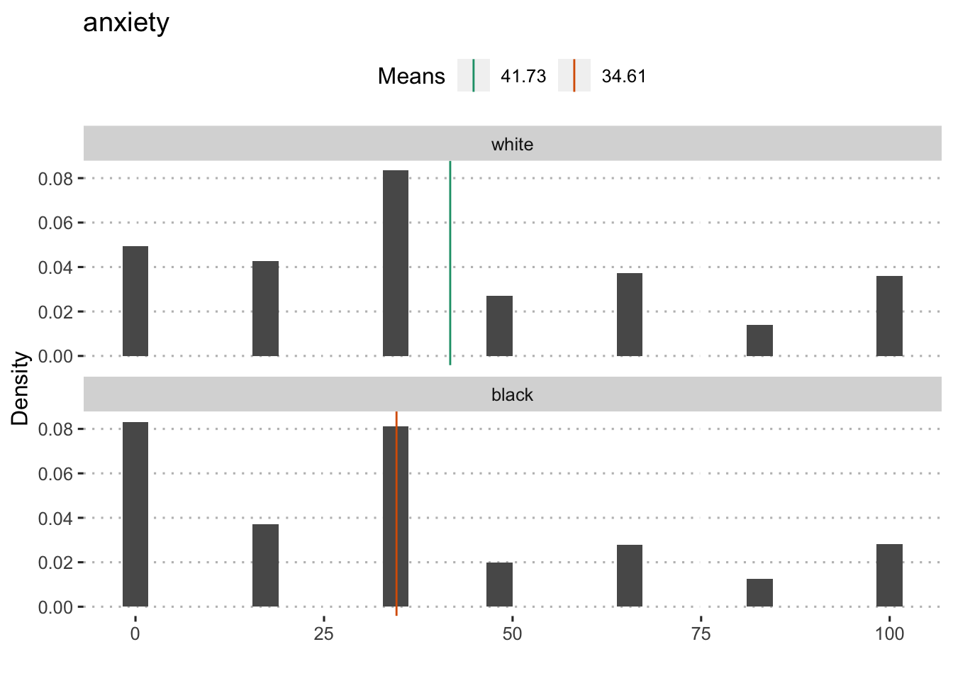
Anxiety
Black
##
## Welch Two Sample t-test
##
## data: anxiety by compare1
## t = 5.8653, df = 957.37, p-value = 6.168e-09
## alternative hypothesis: true difference in means is not equal to 0
## 95 percent confidence interval:
## 4.739698 9.506118
## sample estimates:
## mean in group 0 mean in group 1
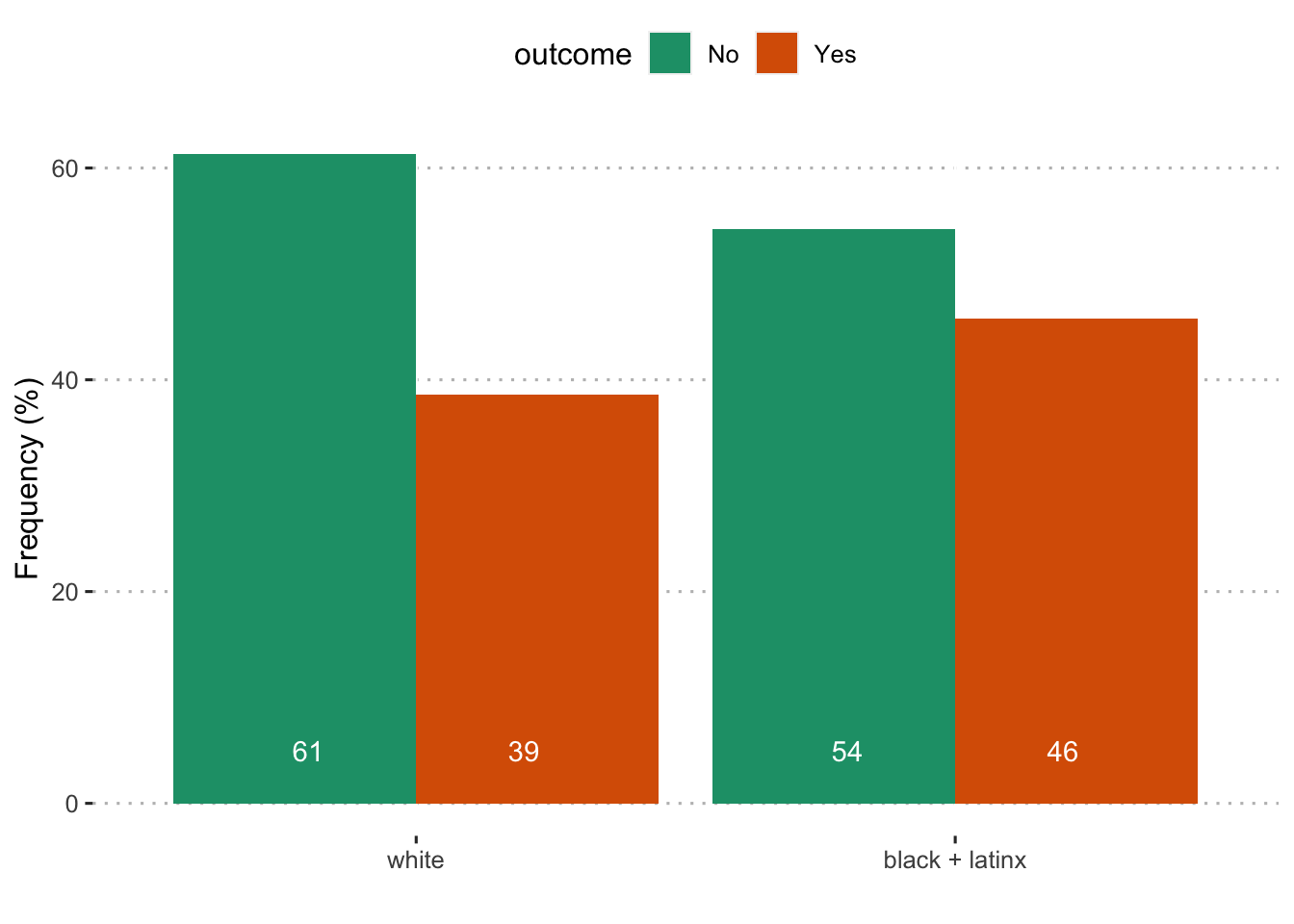
## 41.73164 34.60873Black + LatinX
##
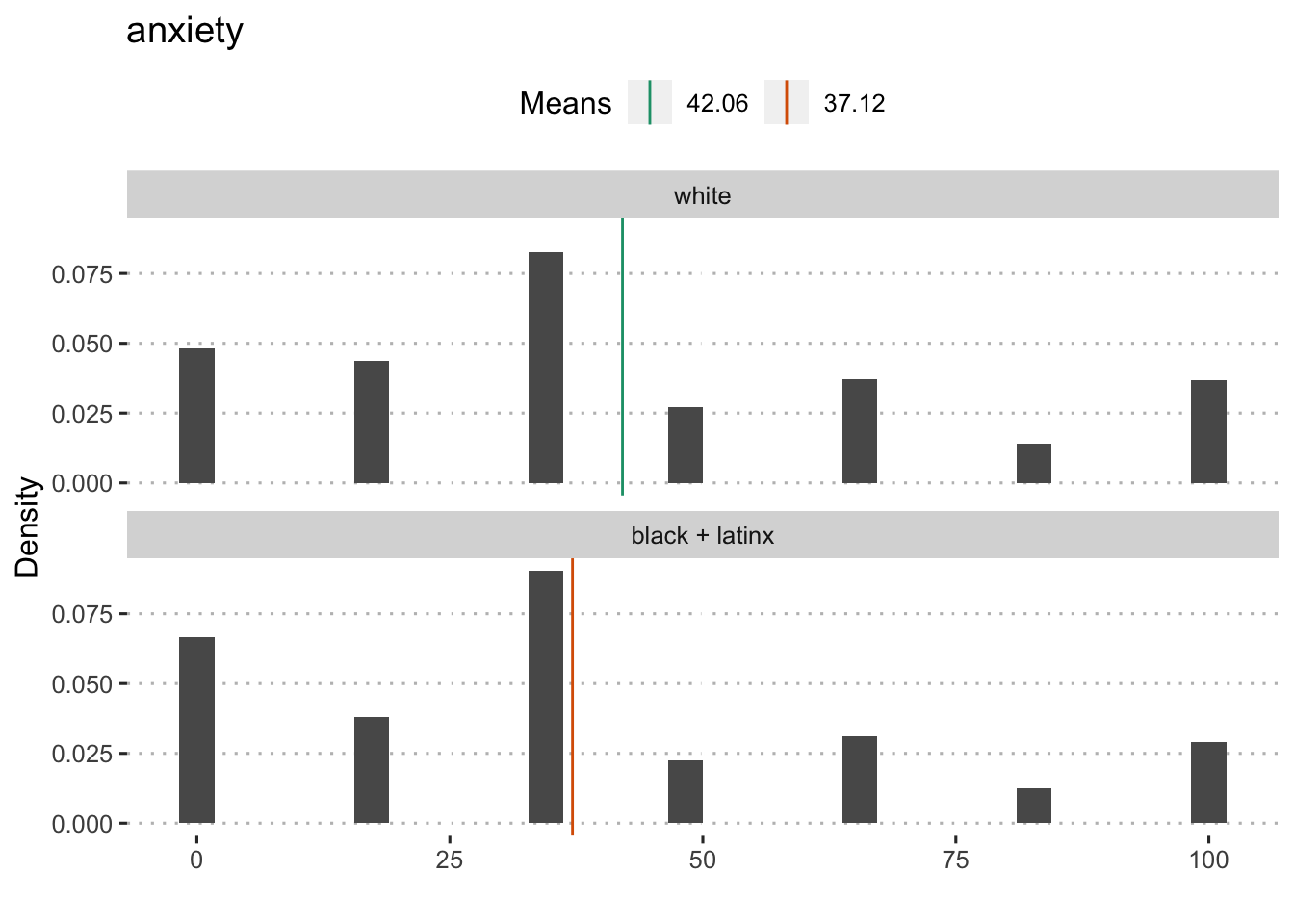
## Welch Two Sample t-test
##
## data: anxiety by compare2
## t = 6.2848, df = 4003, p-value = 3.634e-10
## alternative hypothesis: true difference in means is not equal to 0
## 95 percent confidence interval:
## 3.396554 6.476471
## sample estimates:
## mean in group 0 mean in group 1
## 42.05911 37.12260People of Color (minus Asian)
##
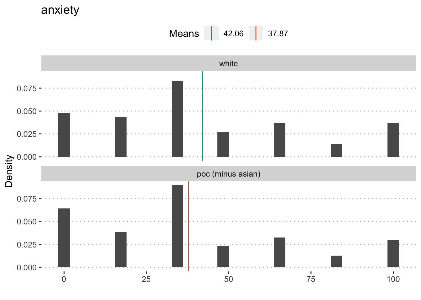
## Welch Two Sample t-test
##
## data: anxiety by compare3
## t = 5.6188, df = 4950.8, p-value = 2.028e-08
## alternative hypothesis: true difference in means is not equal to 0
## 95 percent confidence interval:
## 2.728334 5.652483
## sample estimates:
## mean in group 0 mean in group 1
## 42.05911 37.86870People of Color
##
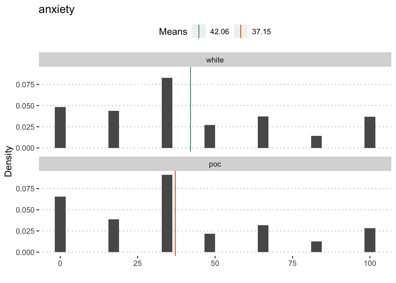
## Welch Two Sample t-test
##
## data: anxiety by compare4
## t = 6.8855, df = 5858.9, p-value = 6.362e-12
## alternative hypothesis: true difference in means is not equal to 0
## 95 percent confidence interval:
## 3.508842 6.302134
## sample estimates:
## mean in group 0 mean in group 1
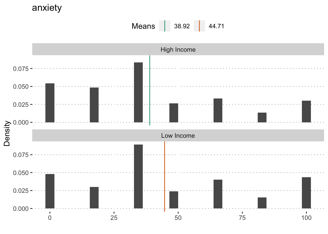
## 42.05911 37.15362By income
## Analysis of Variance Table
##
## Response: anxiety
## Df Sum Sq Mean Sq F value Pr(>F)
## poverty150 1 58223 58223 58.794 1.962e-14 ***
## Residuals 7811 7735119 990
## ---
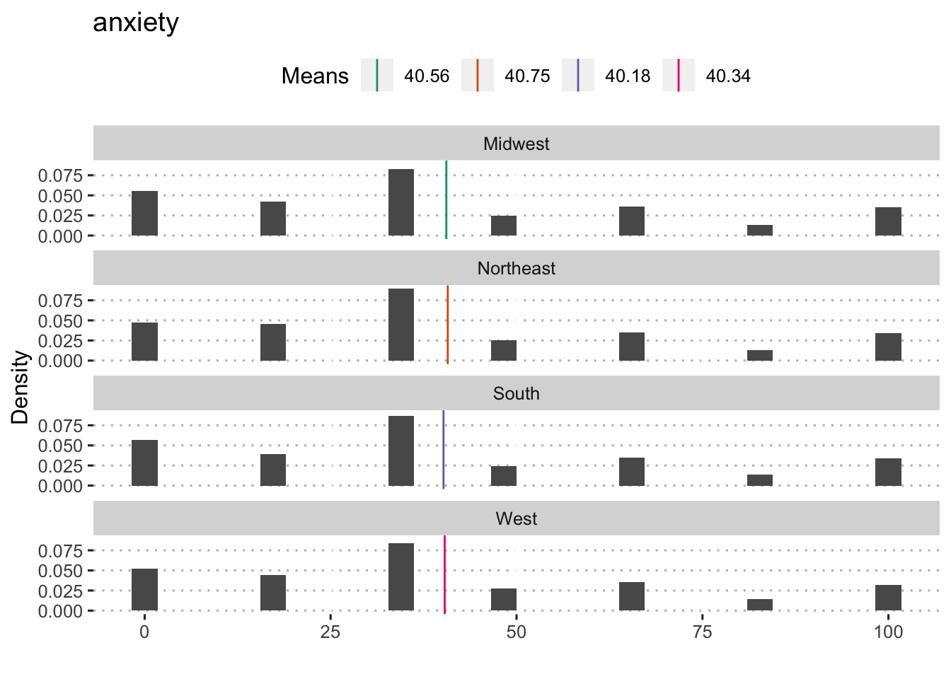
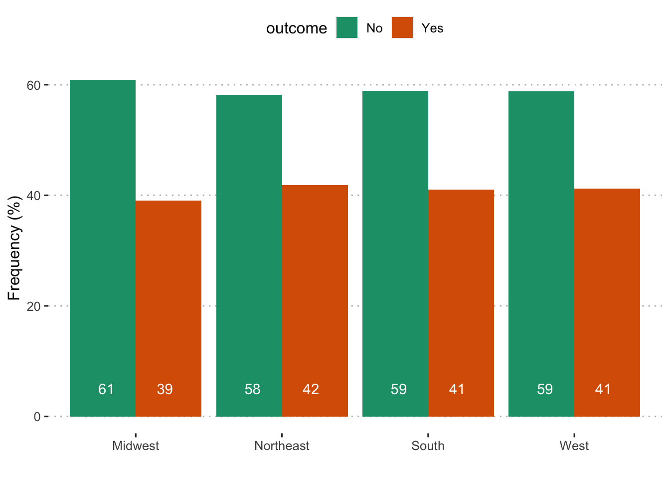
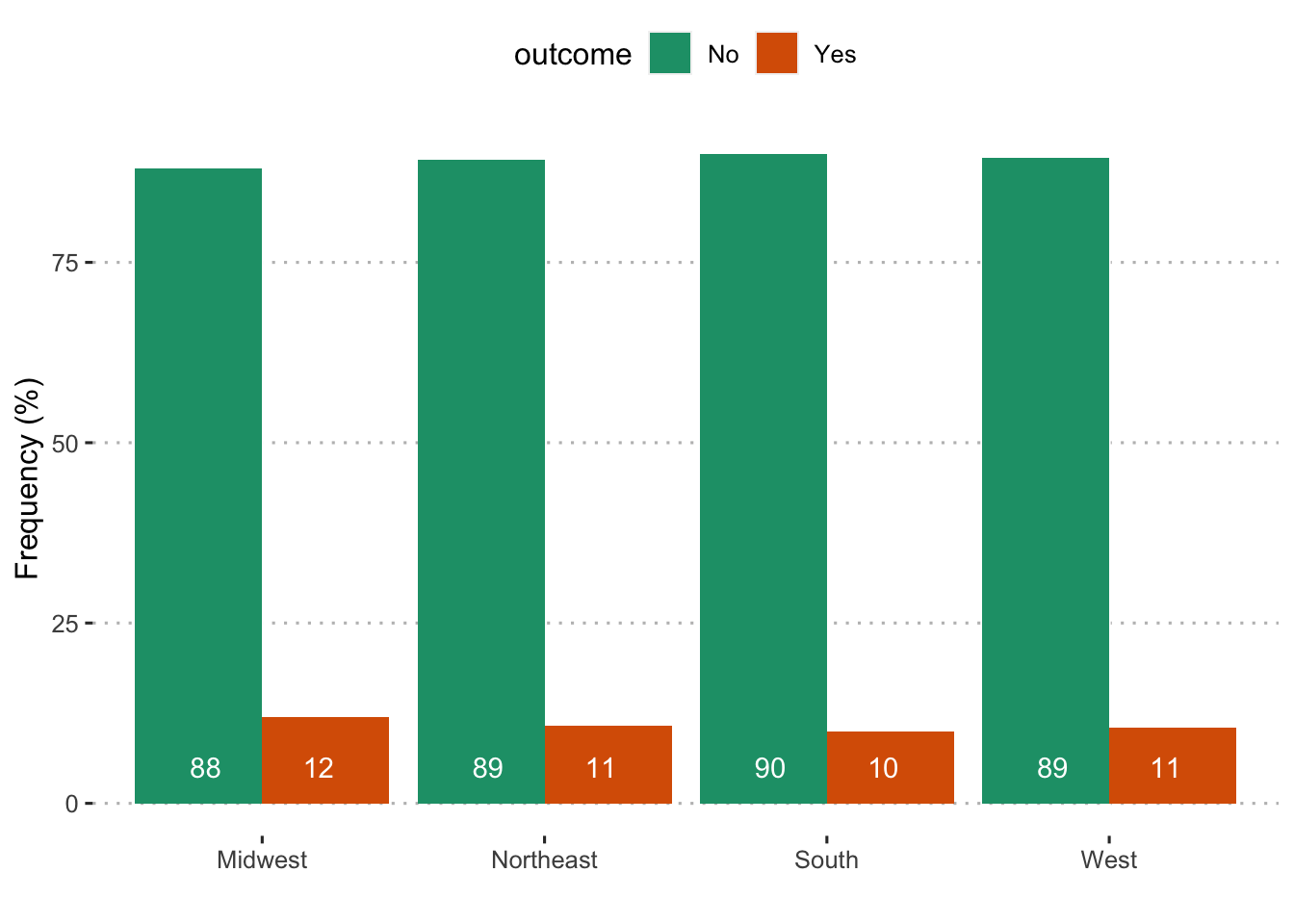
## Signif. codes: 0 '***' 0.001 '**' 0.01 '*' 0.05 '.' 0.1 ' ' 1Geographic Region
## Analysis of Variance Table
##
## Response: anxiety
## Df Sum Sq Mean Sq F value Pr(>F)
## region 3 377 125.63 0.1261 0.9447
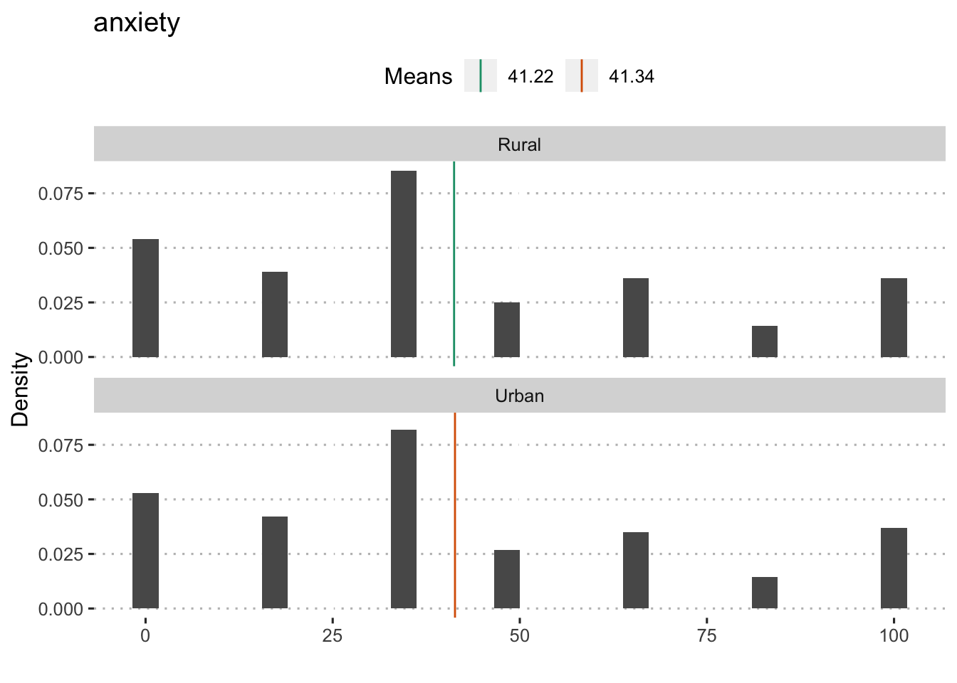
## Residuals 8761 8730421 996.51Rural/Urban
##
## Welch Two Sample t-test
##
## data: anxiety by rural
## t = -0.12772, df = 3755.3, p-value = 0.8984
## alternative hypothesis: true difference in means is not equal to 0
## 95 percent confidence interval:
## -1.910430 1.676755
## sample estimates:
## mean in group rural mean in group urban
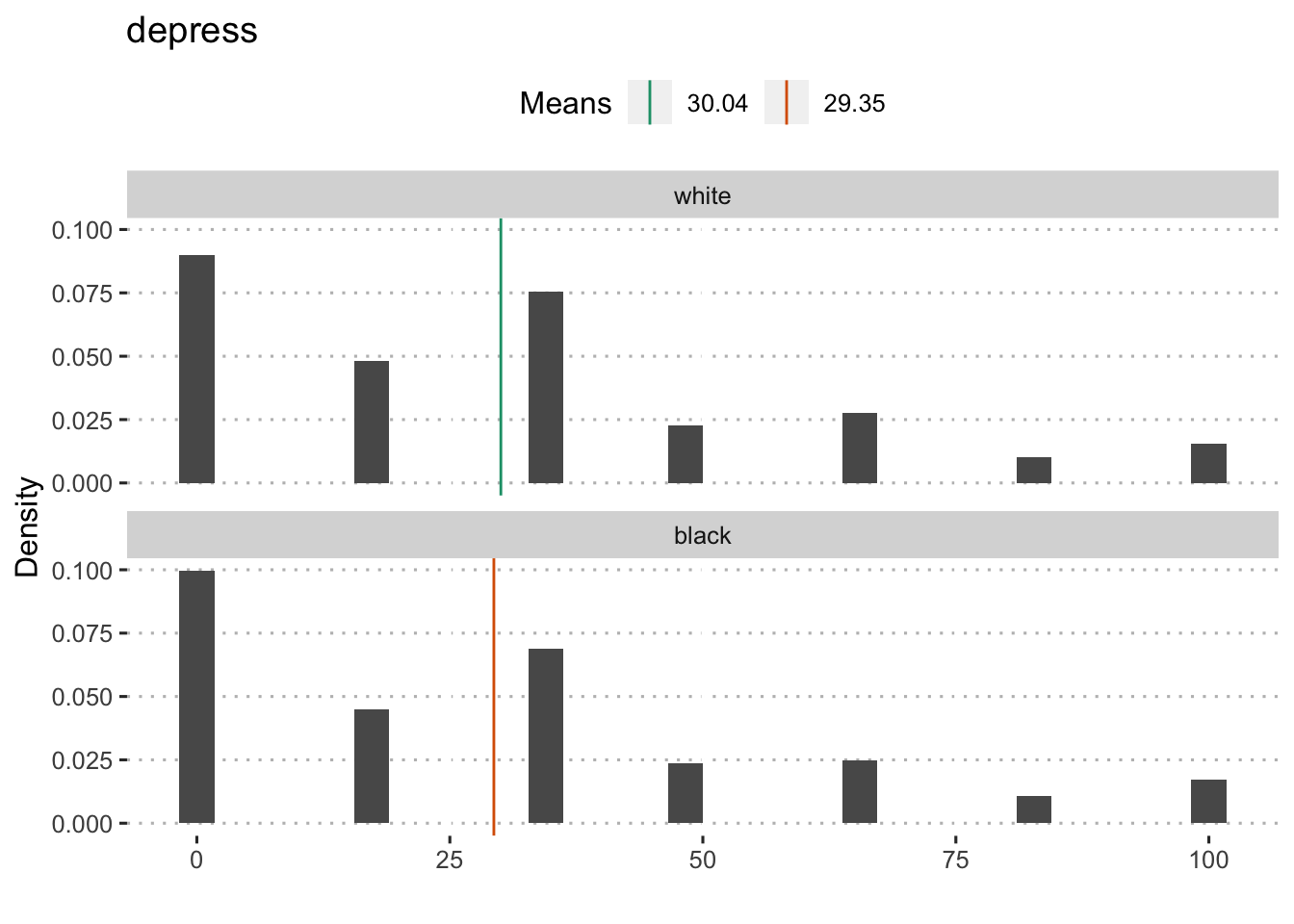
## 41.21829 41.33513Depression
Black
##
##  Welch Two Sample t-test
##
## data:  depress by compare1
## t = 0.61504, df = 946.45, p-value = 0.5387
## alternative hypothesis: true difference in means is not equal to 0
## 95 percent confidence interval:
##  -1.523277  2.913885
## sample estimates:
## mean in group 0 mean in group 1
##        30.04077        29.34547
Black + LatinX
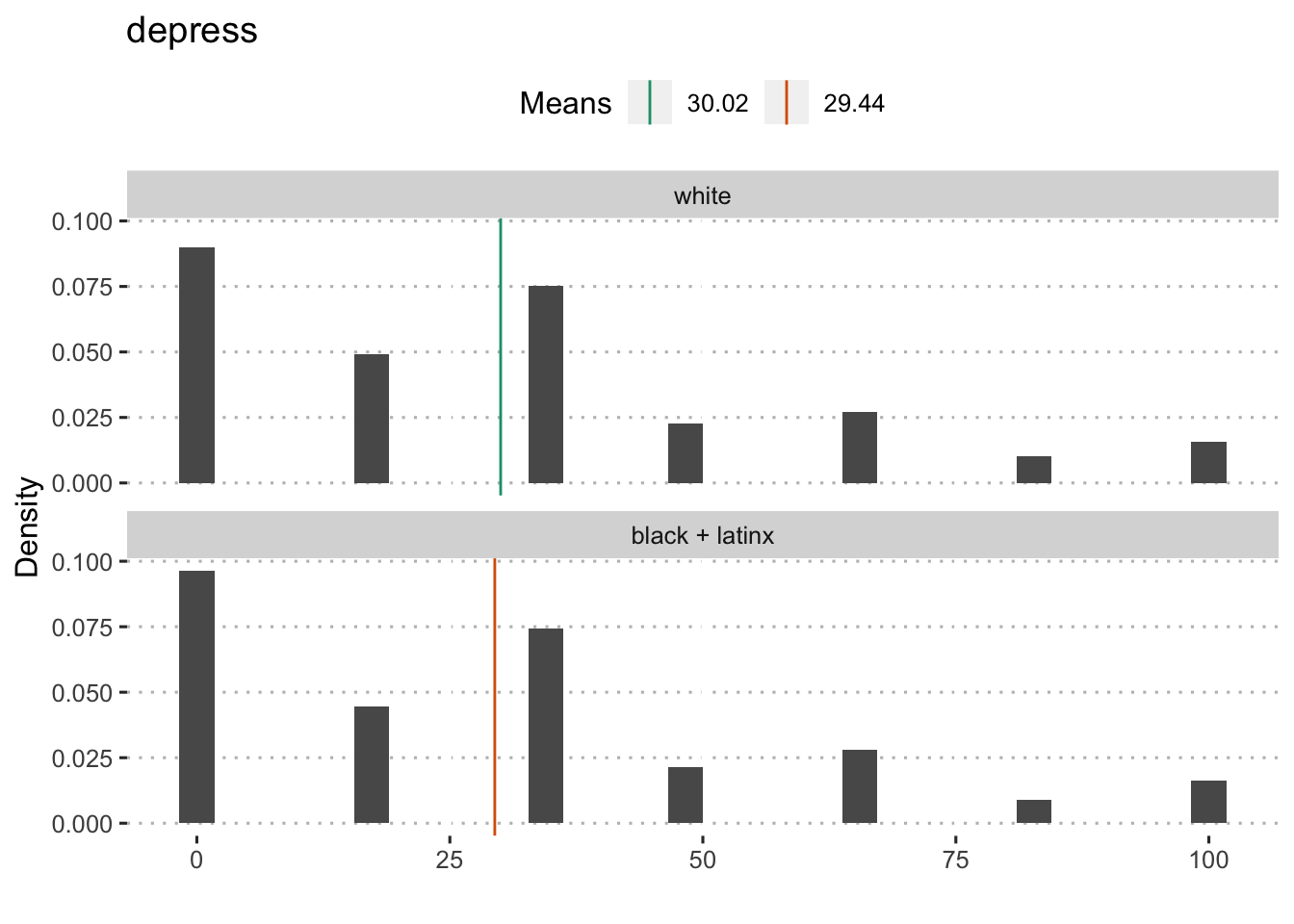
##
##  Welch Two Sample t-test
##
## data:  depress by compare2
## t = 0.79911, df = 3898, p-value = 0.4243
## alternative hypothesis: true difference in means is not equal to 0
## 95 percent confidence interval:
##  -0.8487723  2.0167131
## sample estimates:
## mean in group 0 mean in group 1
##        30.02358        29.43961
People of Color (minus Asian)
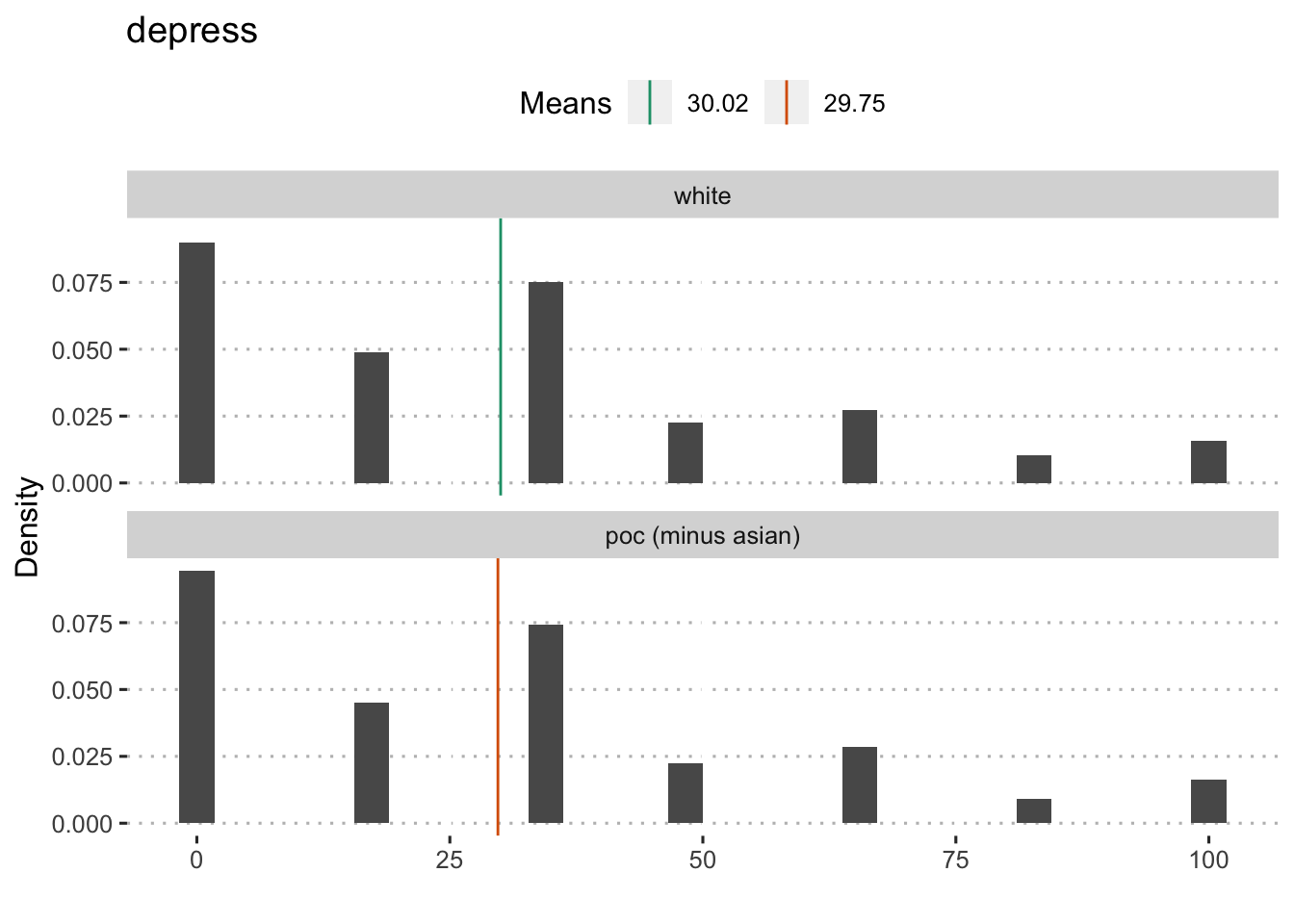
##
##  Welch Two Sample t-test
##
## data:  depress by compare3
## t = 0.39147, df = 4839.9, p-value = 0.6955
## alternative hypothesis: true difference in means is not equal to 0
## 95 percent confidence interval:
##  -1.084310  1.625393
## sample estimates:
## mean in group 0 mean in group 1
##        30.02358        29.75304
People of Color
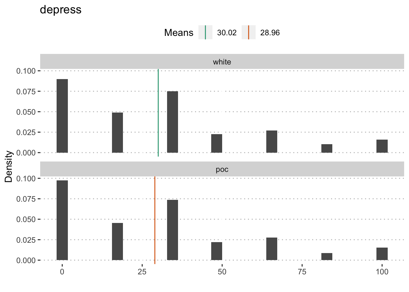
##
##  Welch Two Sample t-test
##
## data:  depress by compare4
## t = 1.6078, df = 5735.7, p-value = 0.1079
## alternative hypothesis: true difference in means is not equal to 0
## 95 percent confidence interval:
##  -0.232457  2.352504
## sample estimates:
## mean in group 0 mean in group 1
##        30.02358        28.96356
By income
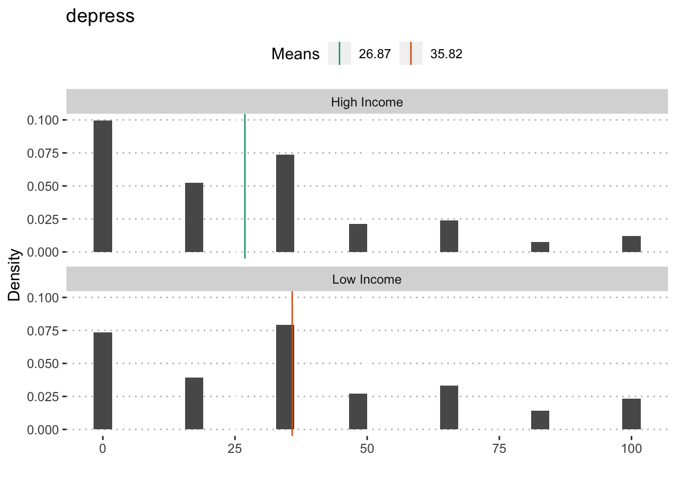
## Analysis of Variance Table
##
## Response: depress
##              Df  Sum Sq Mean Sq F value    Pr(>F)
## poverty150    1  138824  138824  170.14 < 2.2e-16 ***
## Residuals  7809 6371710     816
## ---
## Signif. codes:  0 '***' 0.001 '**' 0.01 '*' 0.05 '.' 0.1 ' ' 1
Geographic Region
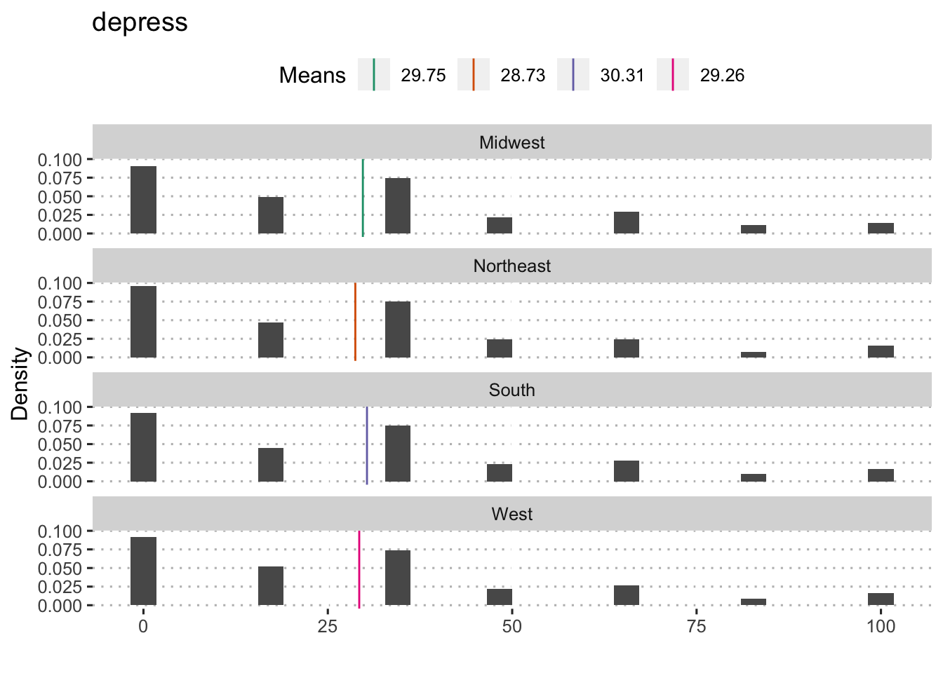
## Analysis of Variance Table
##
## Response: depress
##             Df  Sum Sq Mean Sq F value Pr(>F)
## region       3    2860  953.24  1.1412 0.3309
## Residuals 8757 7314594  835.29
Rural/Urban
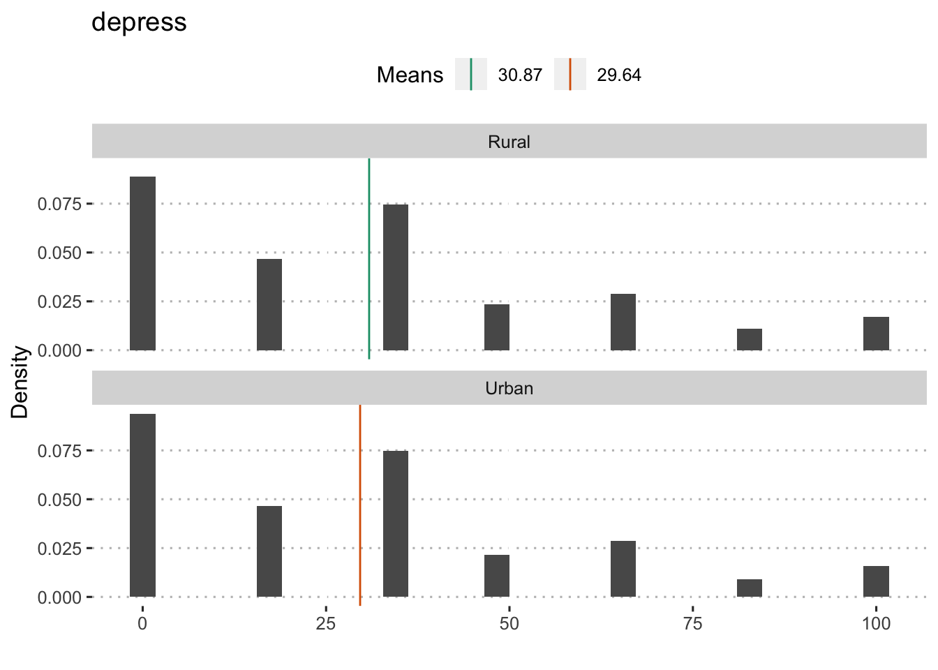
##
##  Welch Two Sample t-test
##
## data:  depress by rural
## t = 1.485, df = 3801.1, p-value = 0.1376
## alternative hypothesis: true difference in means is not equal to 0
## 95 percent confidence interval:
##  -0.396176  2.870366
## sample estimates:
## mean in group rural mean in group urban
##             30.8747             29.6376
Stress
Black
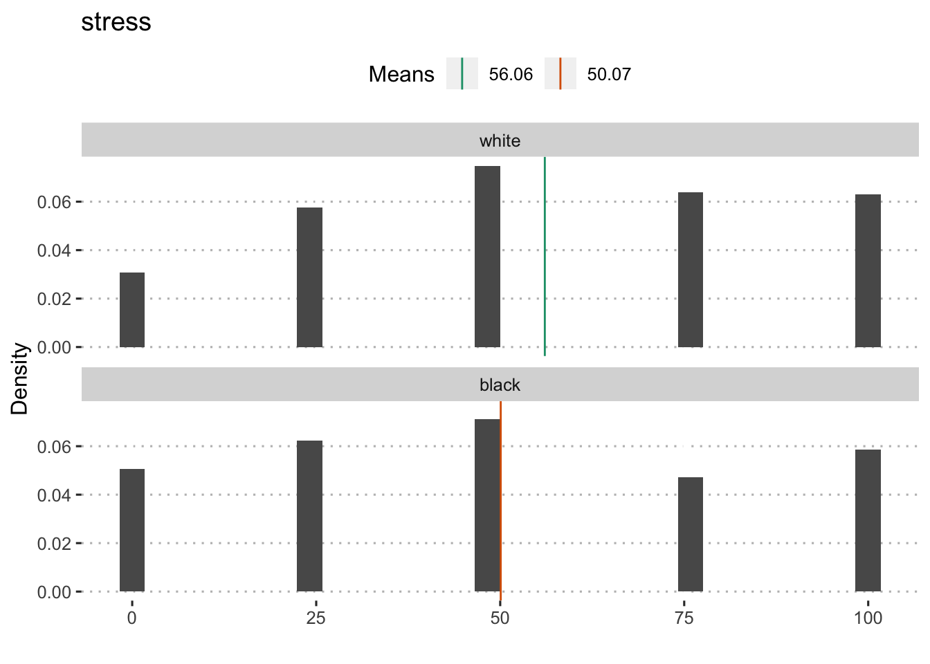
##
##  Welch Two Sample t-test
##
## data:  stress by compare1
## t = 4.5915, df = 924.04, p-value = 5.01e-06
## alternative hypothesis: true difference in means is not equal to 0
## 95 percent confidence interval:
##  3.434278 8.561756
## sample estimates:
## mean in group 0 mean in group 1
##        56.06363        50.06562
Black + LatinX
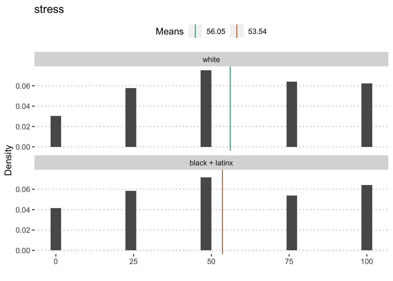
##
##  Welch Two Sample t-test
##
## data:  stress by compare2
## t = 2.9924, df = 3723.1, p-value = 0.002786
## alternative hypothesis: true difference in means is not equal to 0
## 95 percent confidence interval:
##  0.8661328 4.1578448
## sample estimates:
## mean in group 0 mean in group 1
##        56.05049        53.53850
People of Color (minus Asian)

##
##  Welch Two Sample t-test
##
## data:  stress by compare3
## t = 2.1381, df = 4621.6, p-value = 0.03256
## alternative hypothesis: true difference in means is not equal to 0
## 95 percent confidence interval:
##  0.1408149 3.2490806
## sample estimates:
## mean in group 0 mean in group 1
##        56.05049        54.35554
People of Color
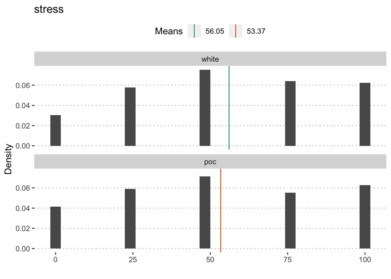
##
##  Welch Two Sample t-test
##
## data:  stress by compare4
## t = 3.53, df = 5443.1, p-value = 0.000419
## alternative hypothesis: true difference in means is not equal to 0
## 95 percent confidence interval:
##  1.190769 4.165283
## sample estimates:
## mean in group 0 mean in group 1
##        56.05049        53.37246
By income
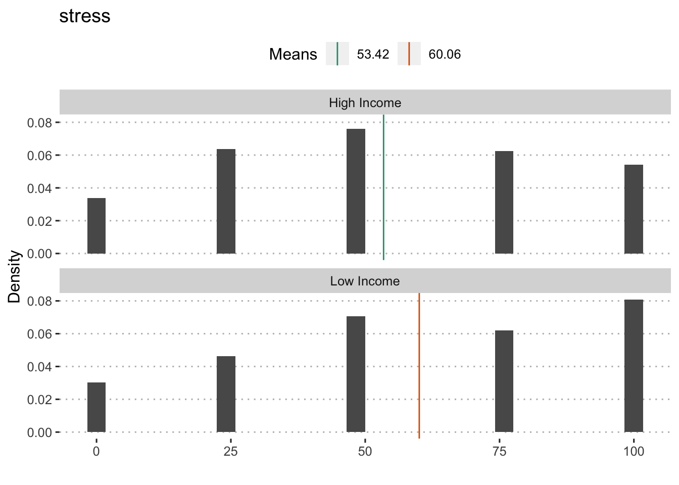
## Analysis of Variance Table
##
## Response: stress
##              Df  Sum Sq Mean Sq F value    Pr(>F)
## poverty150    1   76001   76001  72.926 < 2.2e-16 ***
## Residuals  7758 8085062    1042
## ---
## Signif. codes:  0 '***' 0.001 '**' 0.01 '*' 0.05 '.' 0.1 ' ' 1
Geographic Region
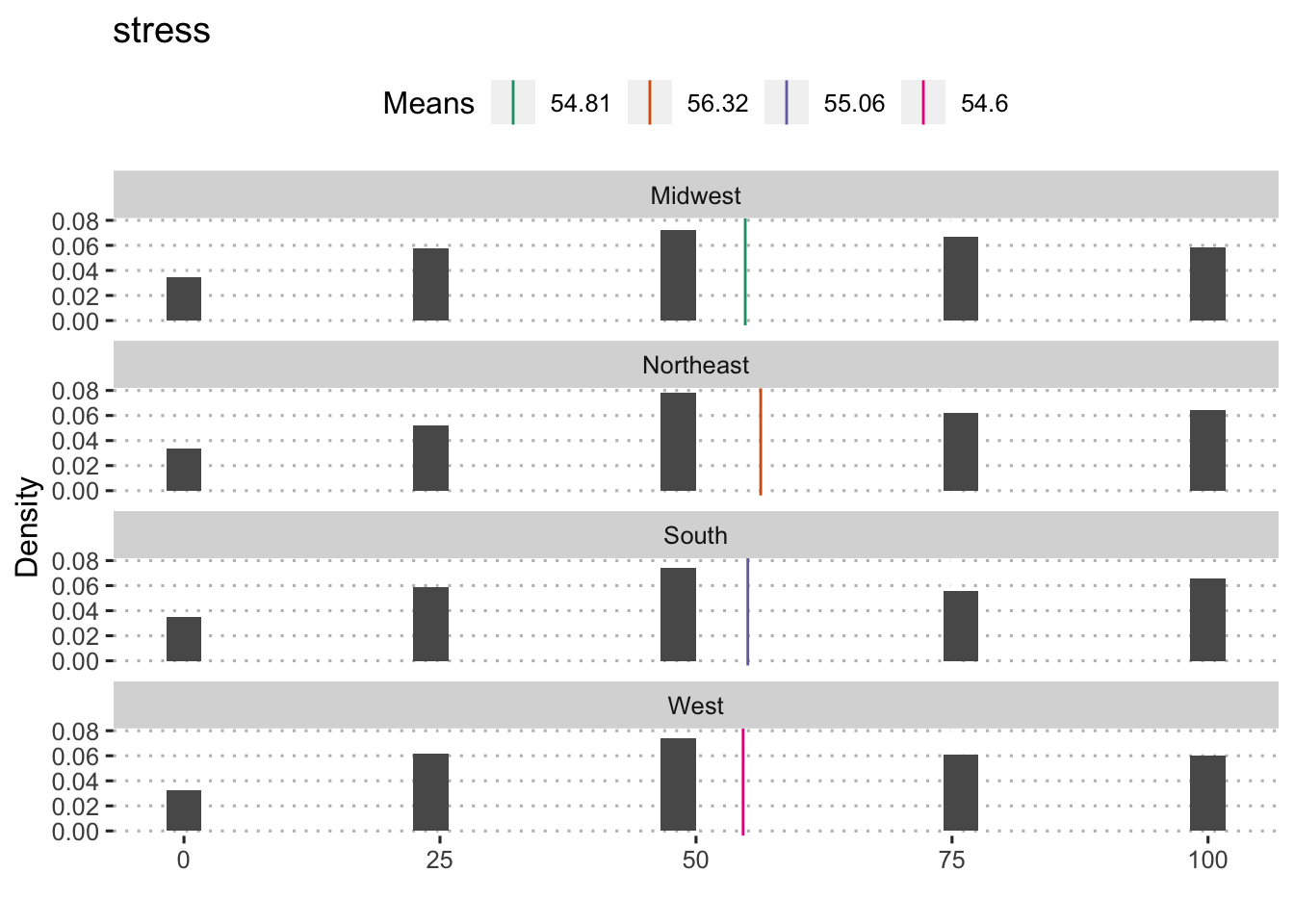
## Analysis of Variance Table
##
## Response: stress
##             Df  Sum Sq Mean Sq F value Pr(>F)
## region       3    2800   933.3  0.8766 0.4523
## Residuals 8707 9270291  1064.7
Rural/Urban
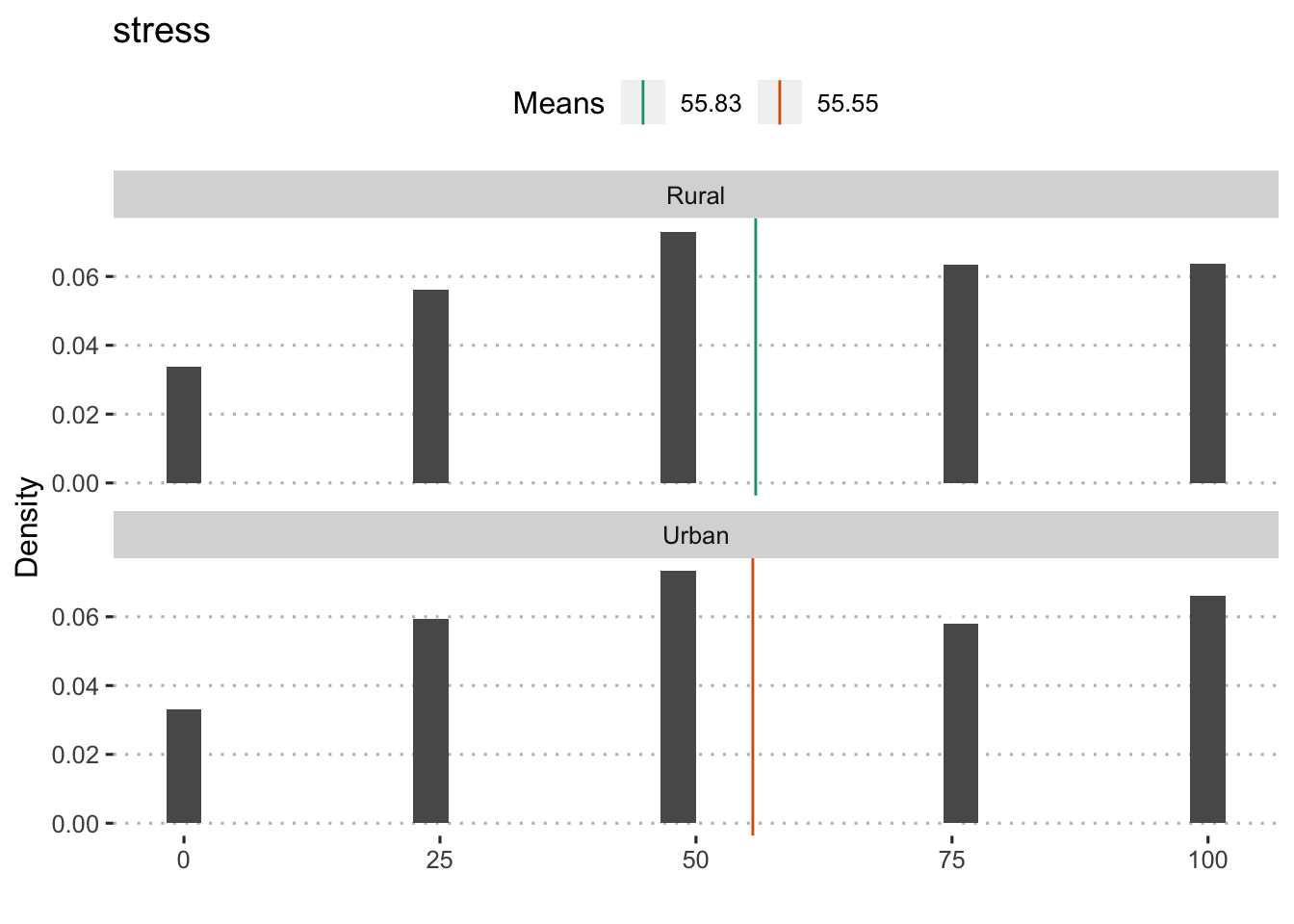
##
## Welch Two Sample t-test
##
## data: stress by rural
## t = 0.295, df = 3722, p-value = 0.768
## alternative hypothesis: true difference in means is not equal to 0
## 95 percent confidence interval:
## -1.563473 2.117292
## sample estimates:
## mean in group rural mean in group urban
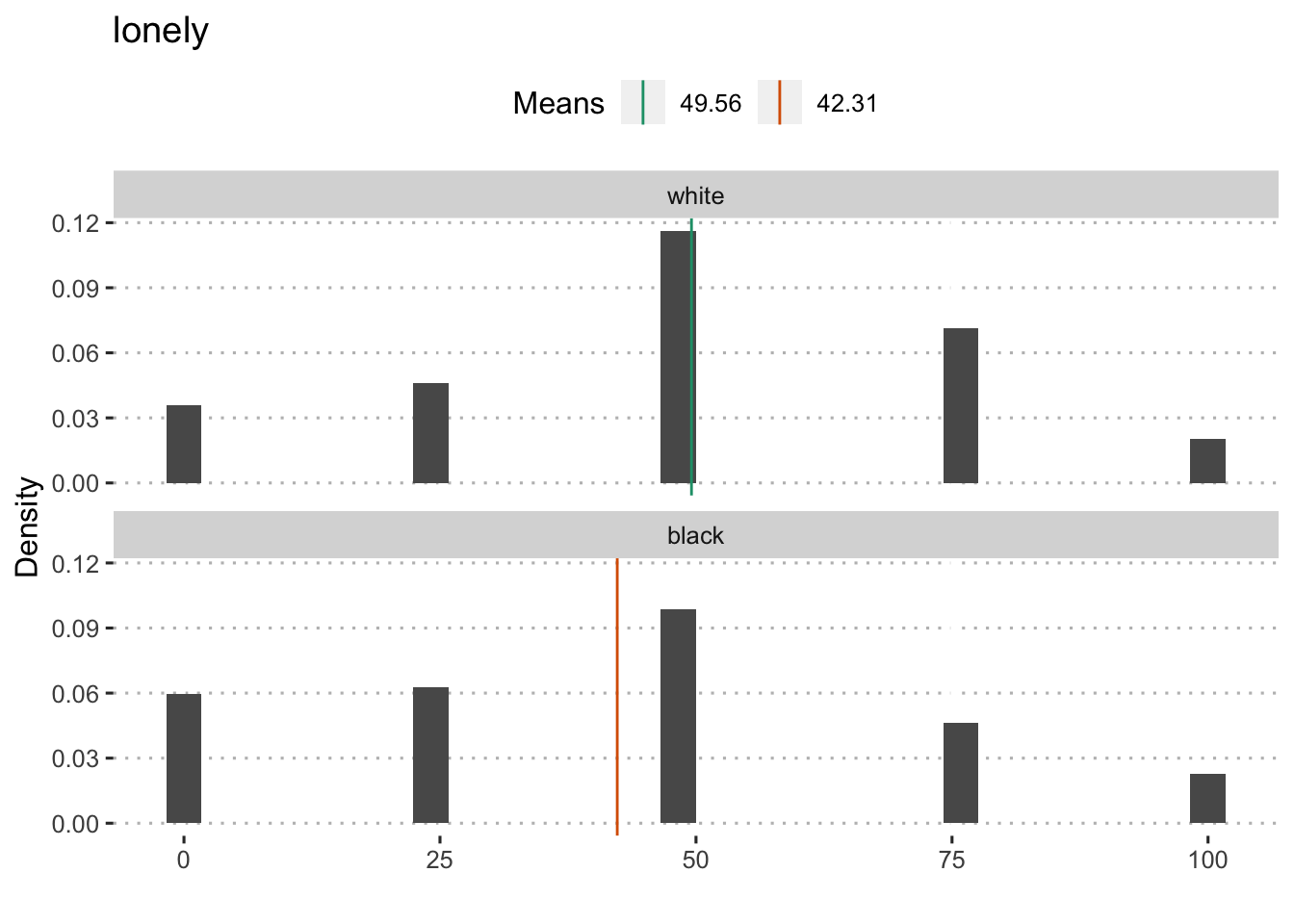
## 55.82796 55.55105Loneliness
Black
##
##  Welch Two Sample t-test
##
## data:  lonely by compare1
## t = 6.4494, df = 925.78, p-value = 1.806e-10
## alternative hypothesis: true difference in means is not equal to 0
## 95 percent confidence interval:
##  5.047386 9.462751
## sample estimates:
## mean in group 0 mean in group 1
##        49.56026        42.30519
Black + LatinX
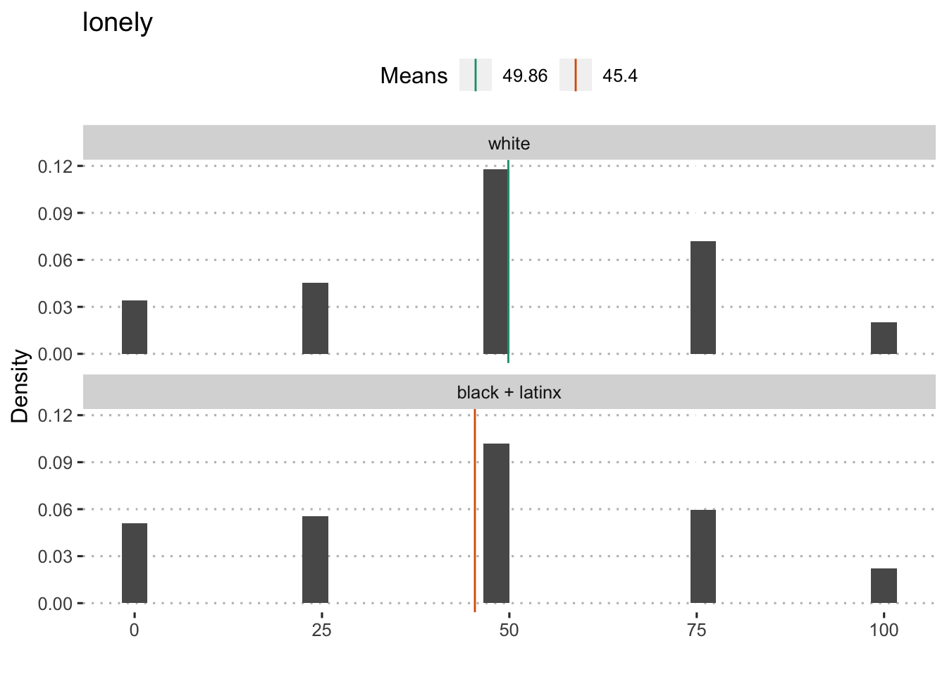
##
##  Welch Two Sample t-test
##
## data:  lonely by compare2
## t = 6.2014, df = 3655.6, p-value = 6.218e-10
## alternative hypothesis: true difference in means is not equal to 0
## 95 percent confidence interval:
##  3.048005 5.866303
## sample estimates:
## mean in group 0 mean in group 1
##        49.85761        45.40046
People of Color (minus Asian)
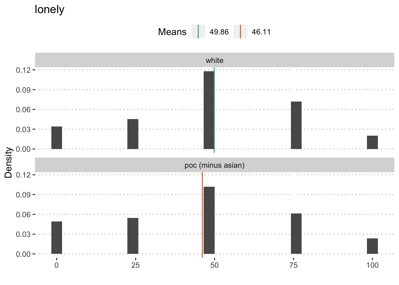
##
##  Welch Two Sample t-test
##
## data:  lonely by compare3
## t = 5.5112, df = 4513.2, p-value = 3.762e-08
## alternative hypothesis: true difference in means is not equal to 0
## 95 percent confidence interval:
##  2.413907 5.079529
## sample estimates:
## mean in group 0 mean in group 1
##        49.85761        46.11089
People of Color
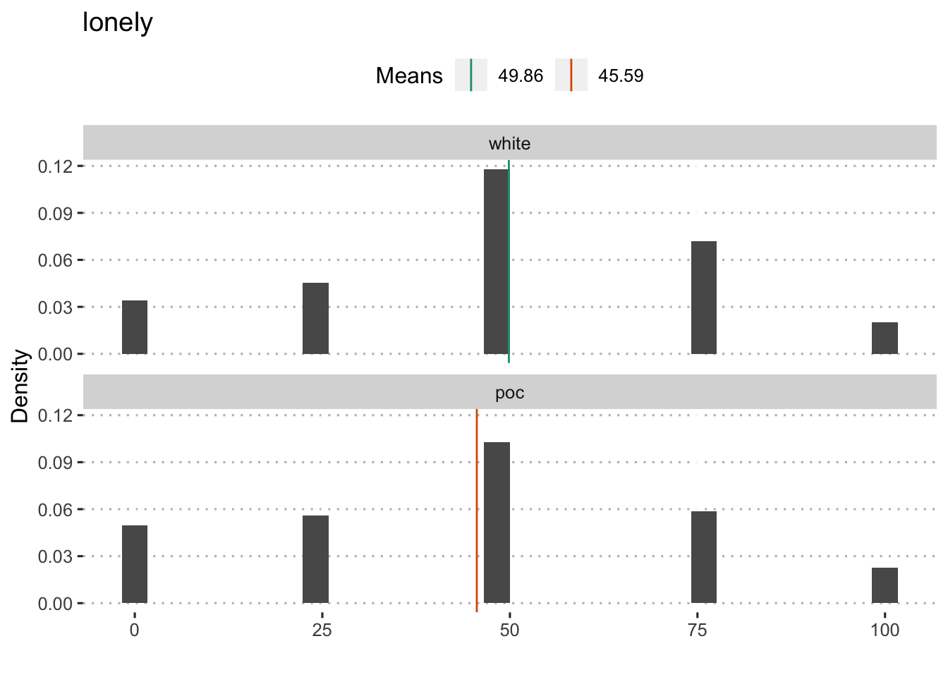
##
##  Welch Two Sample t-test
##
## data:  lonely by compare4
## t = 6.5765, df = 5326.7, p-value = 5.275e-11
## alternative hypothesis: true difference in means is not equal to 0
## 95 percent confidence interval:
##  2.996714 5.542039
## sample estimates:
## mean in group 0 mean in group 1
##        49.85761        45.58824
By income
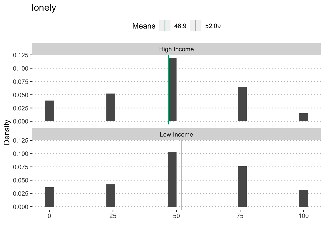
## Analysis of Variance Table
##
## Response: lonely
##              Df  Sum Sq Mean Sq F value    Pr(>F)
## poverty150    1   46774   46774  62.336 3.291e-15 ***
## Residuals  7810 5860239     750
## ---
## Signif. codes:  0 '***' 0.001 '**' 0.01 '*' 0.05 '.' 0.1 ' ' 1
Geographic Region
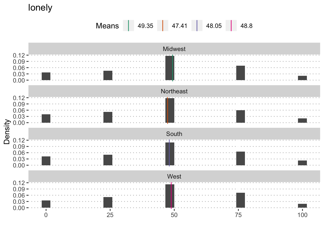
## Analysis of Variance Table
##
## Response: lonely
##             Df  Sum Sq Mean Sq F value Pr(>F)
## region       3    3998 1332.69  1.7376 0.1569
## Residuals 8757 6716295  766.96
Rural/Urban
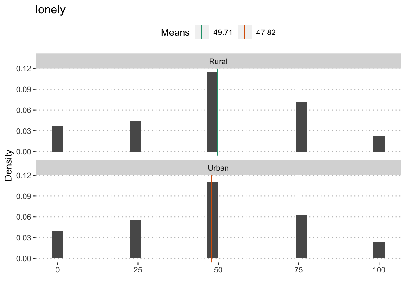
##
##  Welch Two Sample t-test
##
## data:  lonely by rural
## t = 2.3755, df = 3714.2, p-value = 0.01757
## alternative hypothesis: true difference in means is not equal to 0
## 95 percent confidence interval:
##  0.3307875 3.4569118
## sample estimates:
## mean in group rural mean in group urban
##            49.71409            47.82024
Child Externalizing
Black
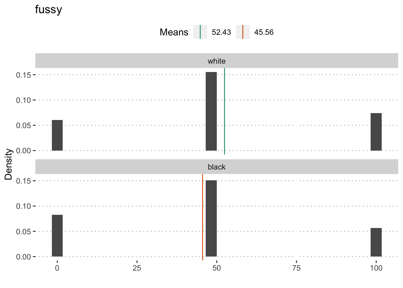
##
##  Welch Two Sample t-test
##
## data:  fussy by compare1
## t = 5.2345, df = 948.51, p-value = 2.037e-07
## alternative hypothesis: true difference in means is not equal to 0
## 95 percent confidence interval:
##  4.292275 9.441015
## sample estimates:
## mean in group 0 mean in group 1
##        52.42800        45.56136
Black + LatinX
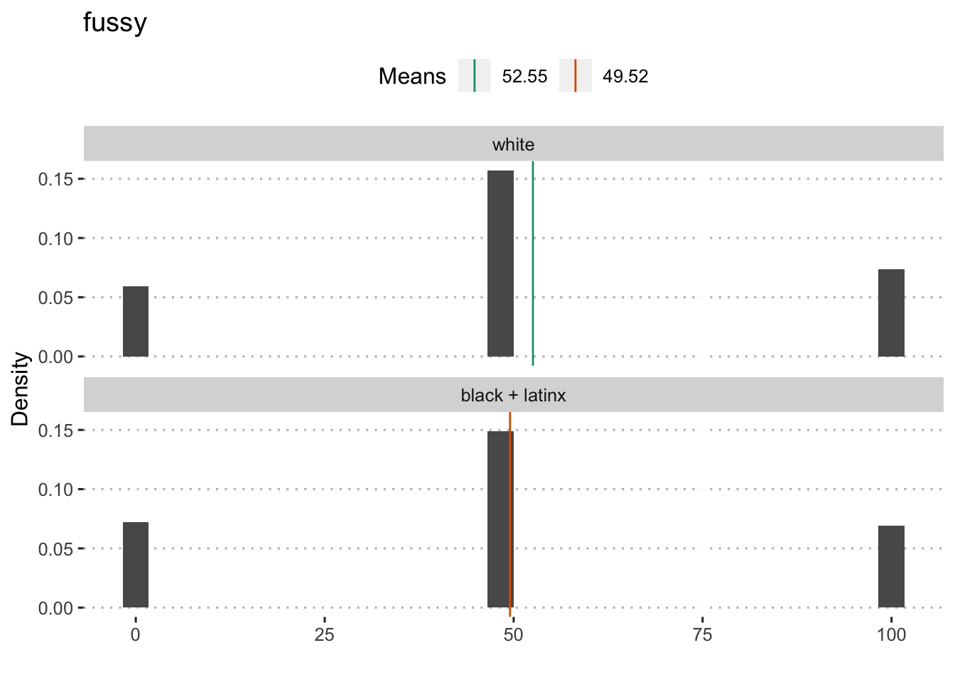
##
##  Welch Two Sample t-test
##
## data:  fussy by compare2
## t = 3.4869, df = 3797.6, p-value = 0.0004943
## alternative hypothesis: true difference in means is not equal to 0
## 95 percent confidence interval:
##  1.327078 4.736509
## sample estimates:
## mean in group 0 mean in group 1
##        52.54926        49.51746
People of Color (minus Asian)
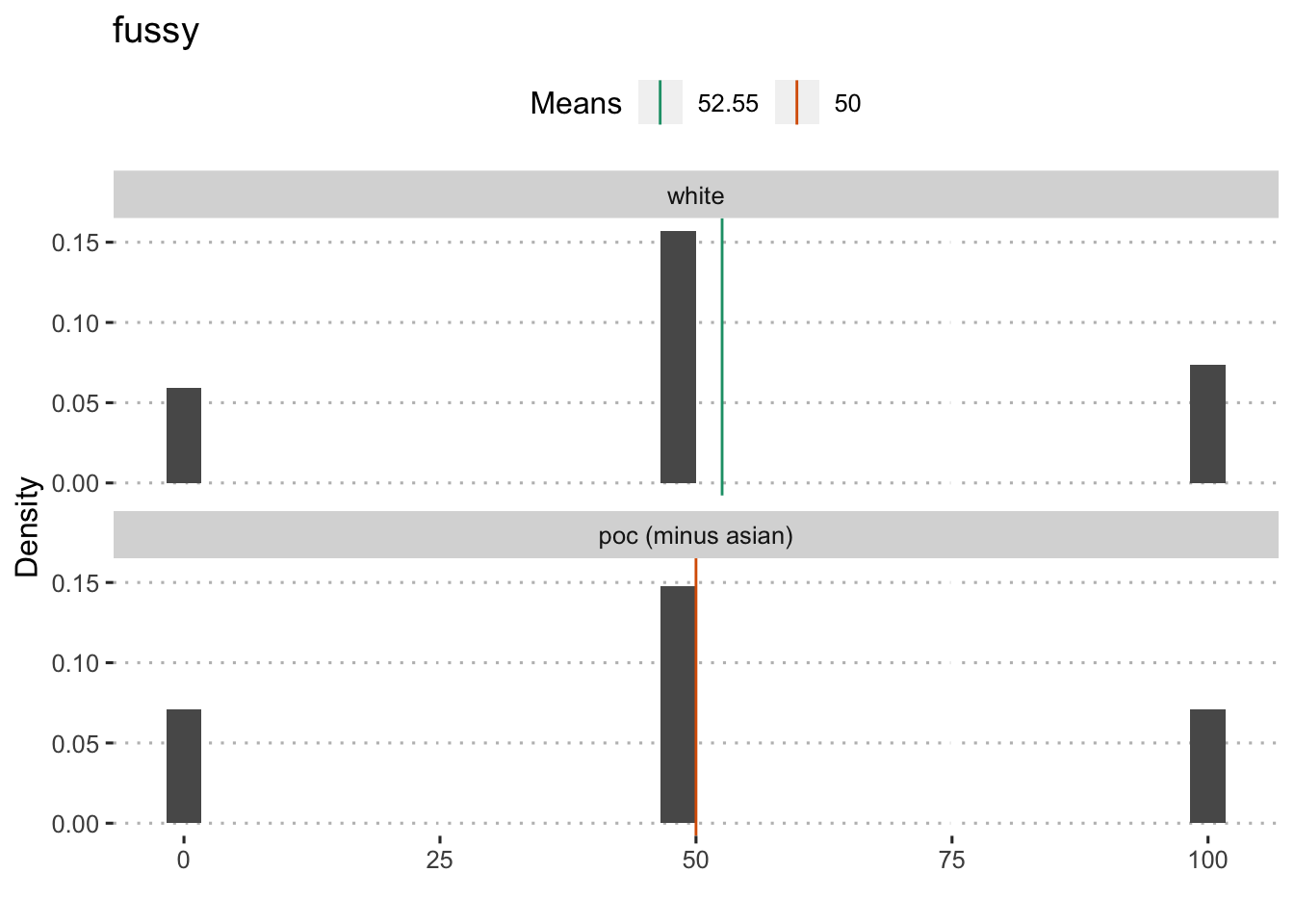
##
##  Welch Two Sample t-test
##
## data:  fussy by compare3
## t = 3.0938, df = 4690.5, p-value = 0.001988
## alternative hypothesis: true difference in means is not equal to 0
## 95 percent confidence interval:
##  0.9338376 4.1646761
## sample estimates:
## mean in group 0 mean in group 1
##        52.54926        50.00000
People of Color

##
##  Welch Two Sample t-test
##
## data:  fussy by compare4
## t = 4.0536, df = 5528.3, p-value = 5.113e-05
## alternative hypothesis: true difference in means is not equal to 0
## 95 percent confidence interval:
##  1.650638 4.742487
## sample estimates:
## mean in group 0 mean in group 1
##        52.54926        49.35269
By income
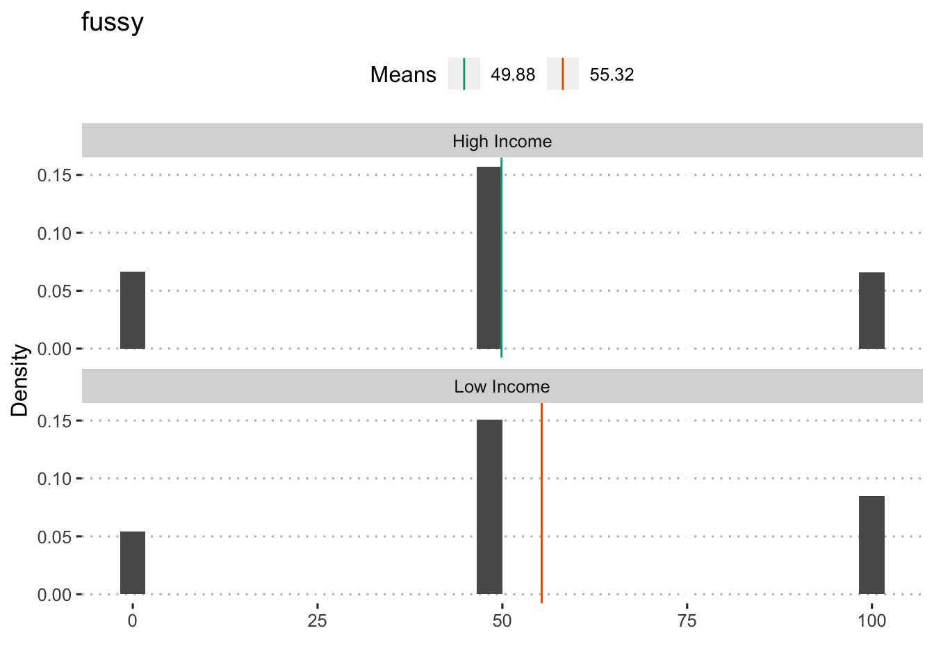
## Analysis of Variance Table
##
## Response: fussy
##              Df  Sum Sq Mean Sq F value    Pr(>F)
## poverty150    1   51018   51018  44.242 3.098e-11 ***
## Residuals  7791 8984293    1153
## ---
## Signif. codes:  0 '***' 0.001 '**' 0.01 '*' 0.05 '.' 0.1 ' ' 1
Geographic Region

## Analysis of Variance Table
##
## Response: fussy
##              Df  Sum Sq Mean Sq F value    Pr(>F)
## poverty150    1   51018   51018  44.242 3.098e-11 ***
## Residuals  7791 8984293    1153
## ---
## Signif. codes:  0 '***' 0.001 '**' 0.01 '*' 0.05 '.' 0.1 ' ' 1
Rural/Urban
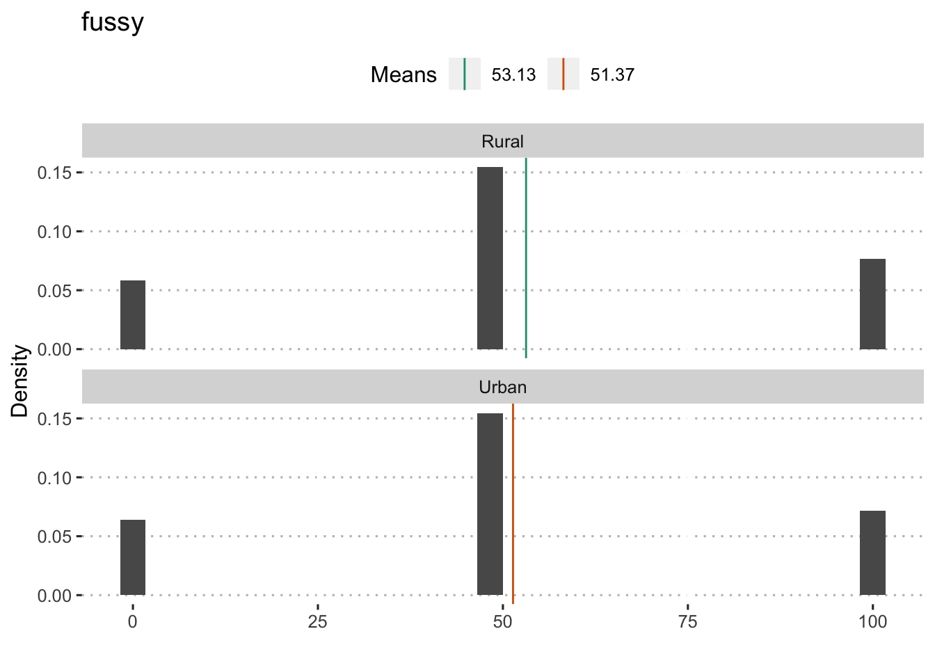
##
## Welch Two Sample t-test
##
## data: fussy by rural
## t = 1.8004, df = 3739.7, p-value = 0.07188
## alternative hypothesis: true difference in means is not equal to 0
## 95 percent confidence interval:
## -0.1562683 3.6689042
## sample estimates:
## mean in group rural mean in group urban
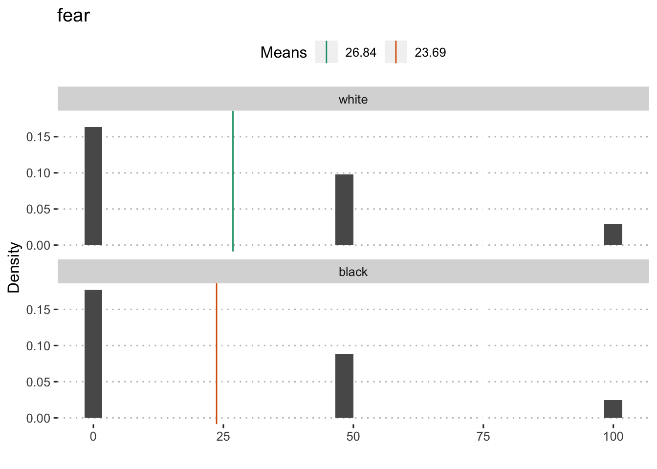
## 53.13024 51.37392Child Internalizing
Black
##
##  Welch Two Sample t-test
##
## data:  fear by compare1
## t = 2.5303, df = 967.79, p-value = 0.01155
## alternative hypothesis: true difference in means is not equal to 0
## 95 percent confidence interval:
##  0.7050749 5.5782944
## sample estimates:
## mean in group 0 mean in group 1
##        26.83620        23.69452
Black + LatinX
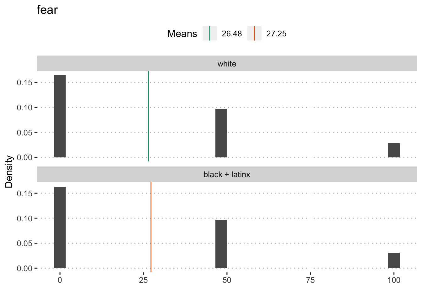
##
##  Welch Two Sample t-test
##
## data:  fear by compare2
## t = -0.90295, df = 3822.2, p-value = 0.3666
## alternative hypothesis: true difference in means is not equal to 0
## 95 percent confidence interval:
##  -2.436724  0.899994
## sample estimates:
## mean in group 0 mean in group 1
##        26.48129        27.24965
People of Color (minus Asian)

##
##  Welch Two Sample t-test
##
## data:  fear by compare3
## t = -1.3103, df = 4723.8, p-value = 0.1902
## alternative hypothesis: true difference in means is not equal to 0
## 95 percent confidence interval:
##  -2.6390822  0.5246155
## sample estimates:
## mean in group 0 mean in group 1
##        26.48129        27.53852
People of Color
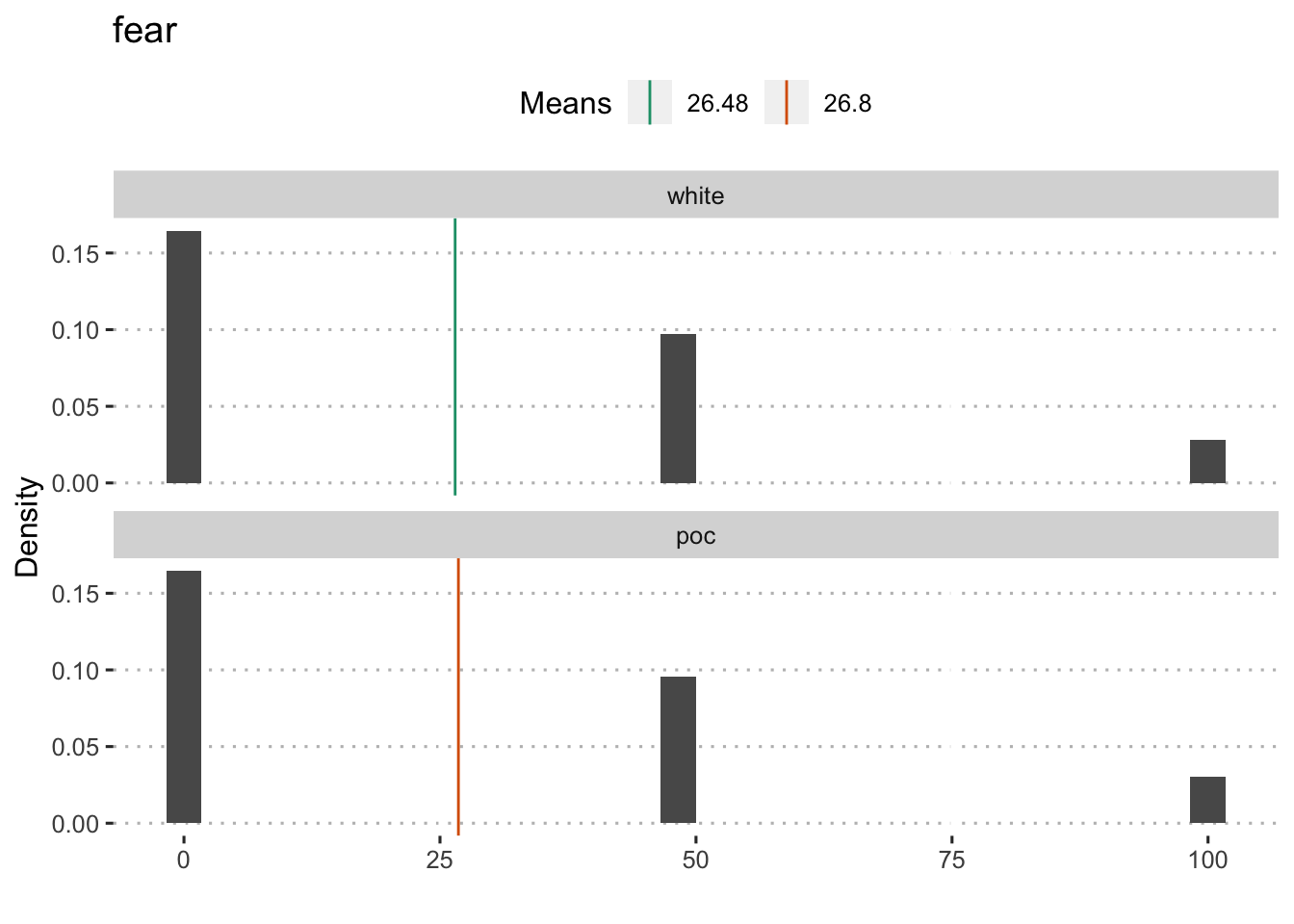
##
## Welch Two Sample t-test
##
## data: fear by compare4
## t = -0.41279, df = 5598.5, p-value = 0.6798
## alternative hypothesis: true difference in means is not equal to 0
## 95 percent confidence interval:
## -1.825851 1.190675
## sample estimates:
## mean in group 0 mean in group 1
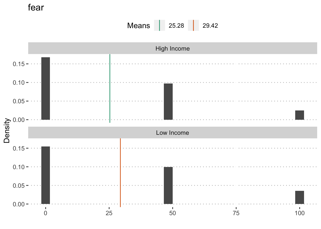
## 26.48129 26.79888By income

## Analysis of Variance Table
##
## Response: fear
##              Df  Sum Sq Mean Sq F value    Pr(>F)
## poverty150    1   29558 29557.7   26.73 2.398e-07 ***
## Residuals  7780 8602974  1105.8
## ---
## Signif. codes:  0 '***' 0.001 '**' 0.01 '*' 0.05 '.' 0.1 ' ' 1
Geographic Region
## Analysis of Variance Table
##
## Response: fear
##              Df  Sum Sq Mean Sq F value    Pr(>F)
## poverty150    1   29558 29557.7   26.73 2.398e-07 ***
## Residuals  7780 8602974  1105.8
## ---
## Signif. codes:  0 '***' 0.001 '**' 0.01 '*' 0.05 '.' 0.1 ' ' 1
Rural/Urban
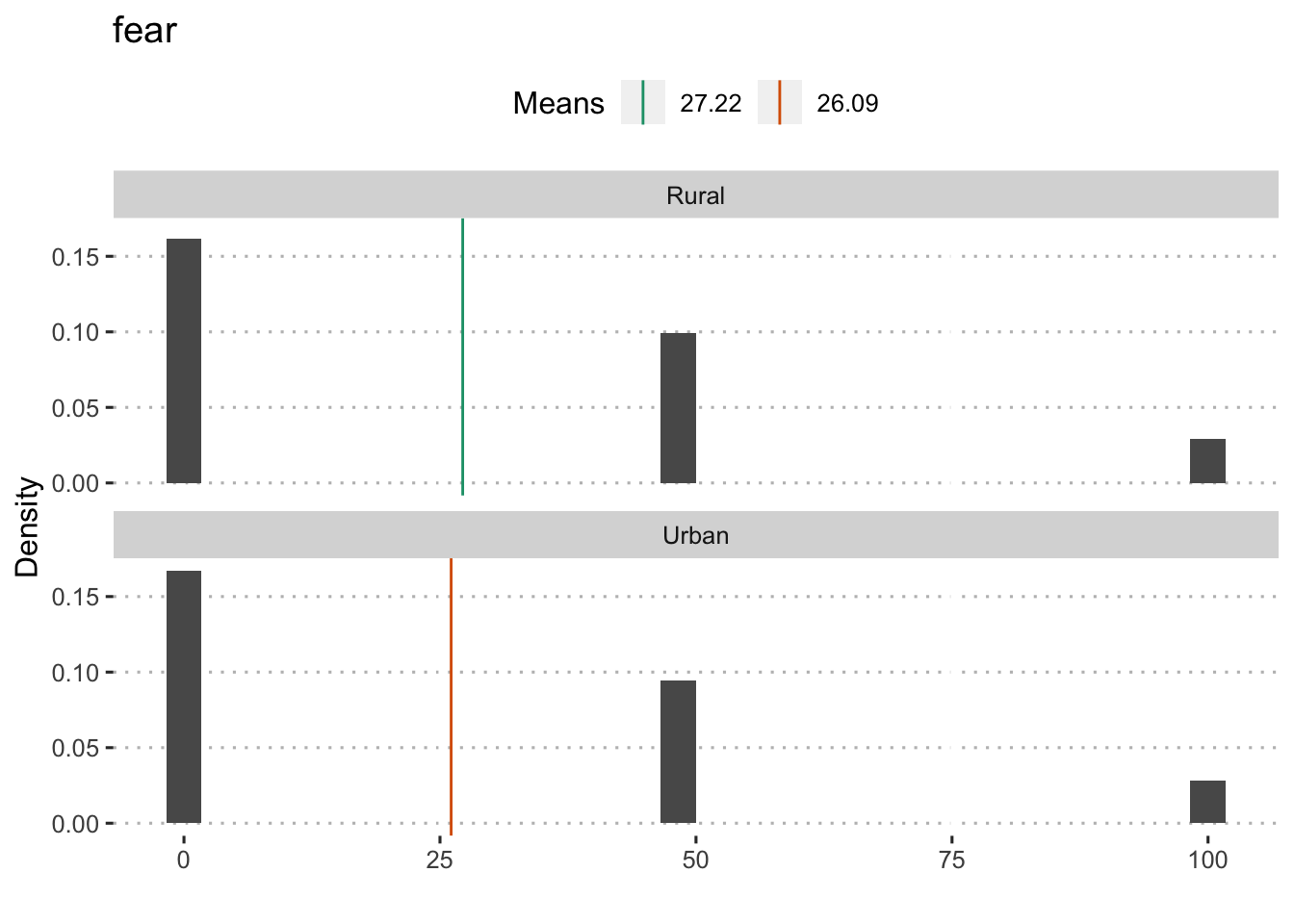
##
##  Welch Two Sample t-test
##
## data:  fear by rural
## t = 1.1802, df = 3773.5, p-value = 0.238
## alternative hypothesis: true difference in means is not equal to 0
## 95 percent confidence interval:
##  -0.7472624  3.0076203
## sample estimates:
## mean in group rural mean in group urban
##            27.22300            26.09282
Work benefits
Income
Black

##
##  Welch Two Sample t-test
##
## data:  income by compare1
## t = 2.4216, df = 755.97, p-value = 0.01569
## alternative hypothesis: true difference in means is not equal to 0
## 95 percent confidence interval:
##   5164.122 49382.310
## sample estimates:
## mean in group 0 mean in group 1
##        88849.34        61576.13
Black + LatinX
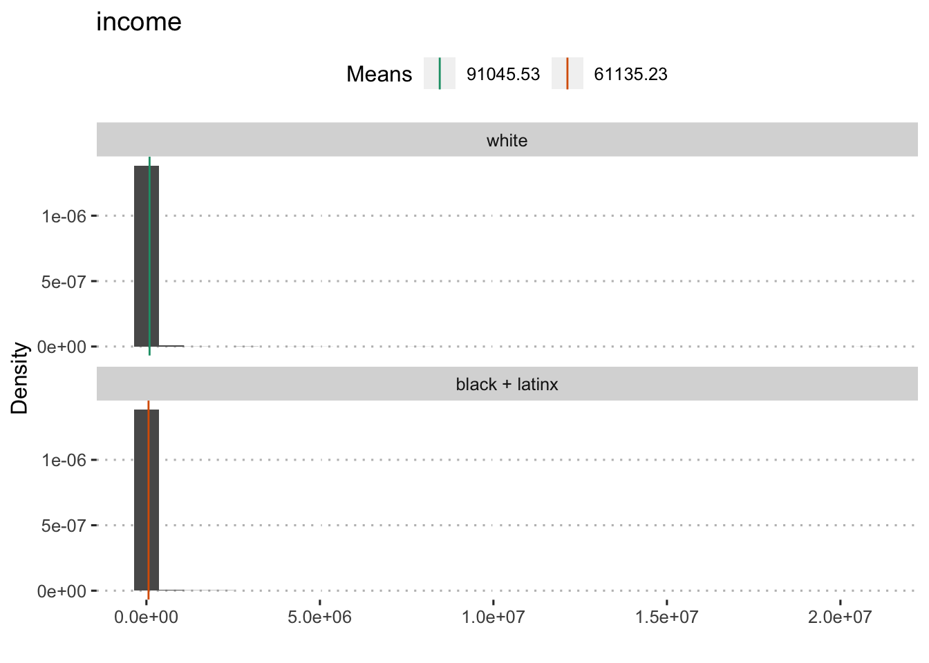
##
##  Welch Two Sample t-test
##
## data:  income by compare2
## t = 3.4932, df = 3904, p-value = 0.0004827
## alternative hypothesis: true difference in means is not equal to 0
## 95 percent confidence interval:
##  13122.79 46697.80
## sample estimates:
## mean in group 0 mean in group 1
##        91045.53        61135.23
People of Color (minus Asian)

##
##  Welch Two Sample t-test
##
## data:  income by compare3
## t = 3.7733, df = 3904.6, p-value = 0.0001635
## alternative hypothesis: true difference in means is not equal to 0
## 95 percent confidence interval:
##  15161.87 47959.16
## sample estimates:
## mean in group 0 mean in group 1
##        91045.53        59485.01
People of Color
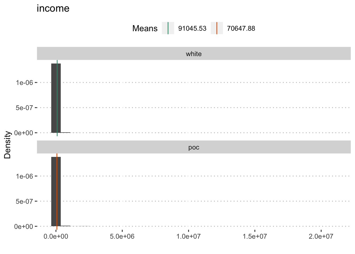
##
##  Welch Two Sample t-test
##
## data:  income by compare4
## t = 2.3625, df = 4131, p-value = 0.0182
## alternative hypothesis: true difference in means is not equal to 0
## 95 percent confidence interval:
##   3470.649 37324.641
## sample estimates:
## mean in group 0 mean in group 1
##        91045.53        70647.88
Geographic Region
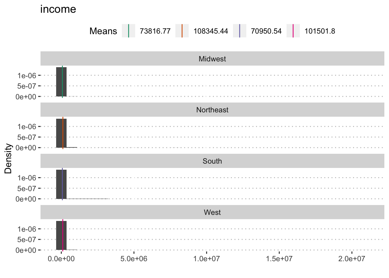
## Analysis of Variance Table
##
## Response: income
##             Df     Sum Sq    Mean Sq F value  Pr(>F)
## region       3 1.0970e+12 3.6567e+11  2.6299 0.04848 *
## Residuals 4273 5.9412e+14 1.3904e+11
## ---
## Signif. codes:  0 '***' 0.001 '**' 0.01 '*' 0.05 '.' 0.1 ' ' 1
Rural/Urban
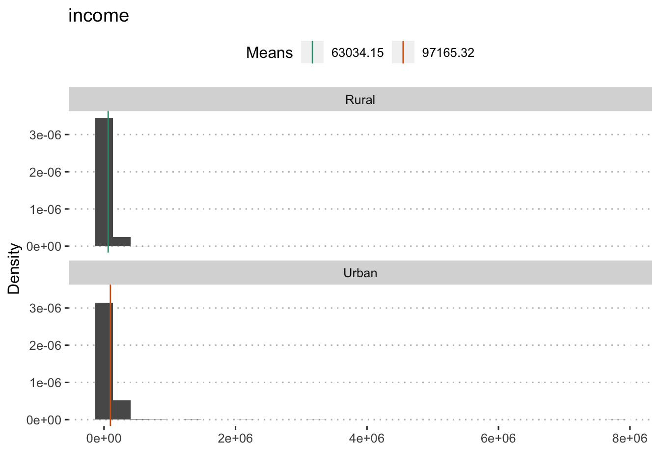
##
##  Welch Two Sample t-test
##
## data:  income by rural
## t = -3.2647, df = 952.12, p-value = 0.001135
## alternative hypothesis: true difference in means is not equal to 0
## 95 percent confidence interval:
##  -54647.98 -13614.37
## sample estimates:
## mean in group rural mean in group urban
##            63034.15            97165.32
Sick Leave
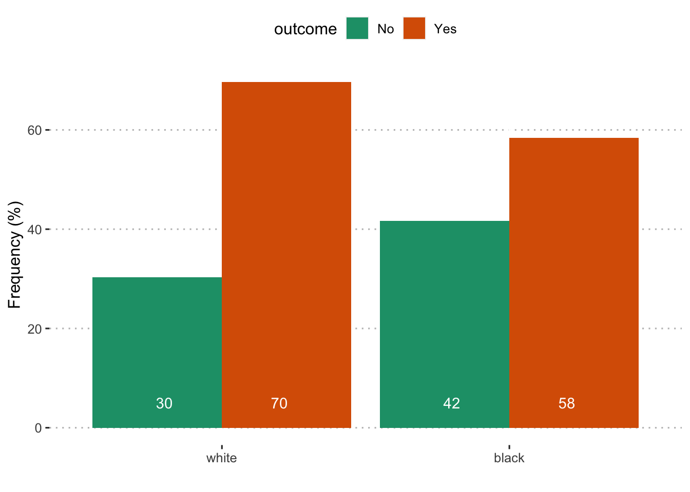
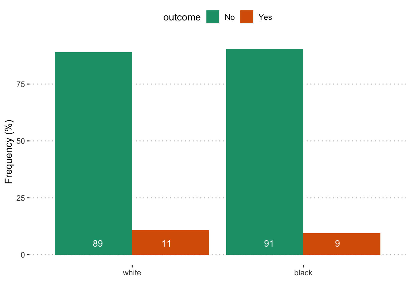
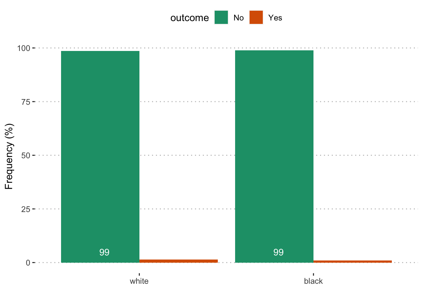
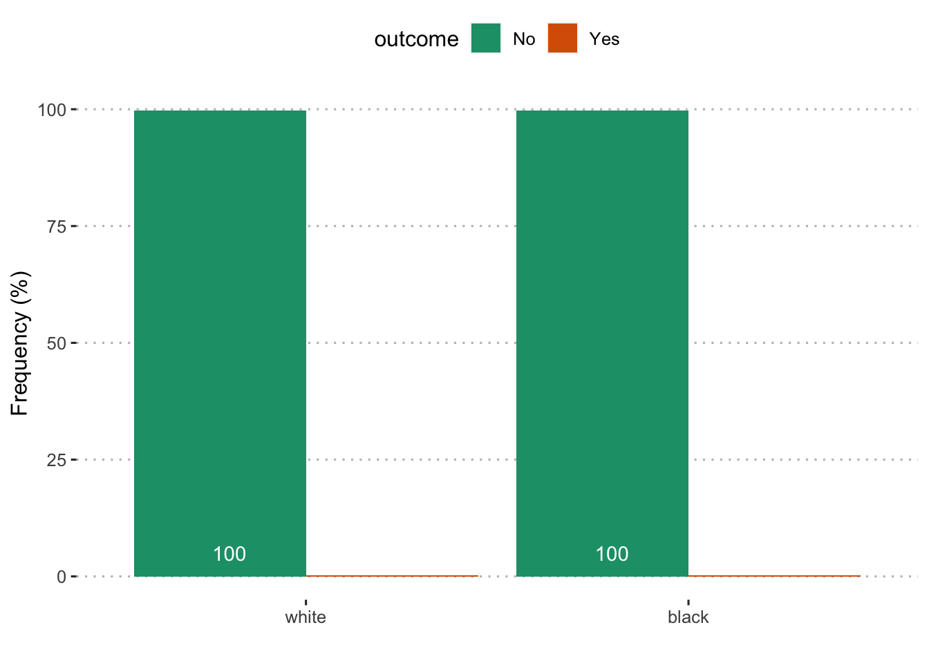
Black
##
## Pearson's Chi-squared test with Yates' continuity correction
##
## data: scored$sick_leave and scored$compare1
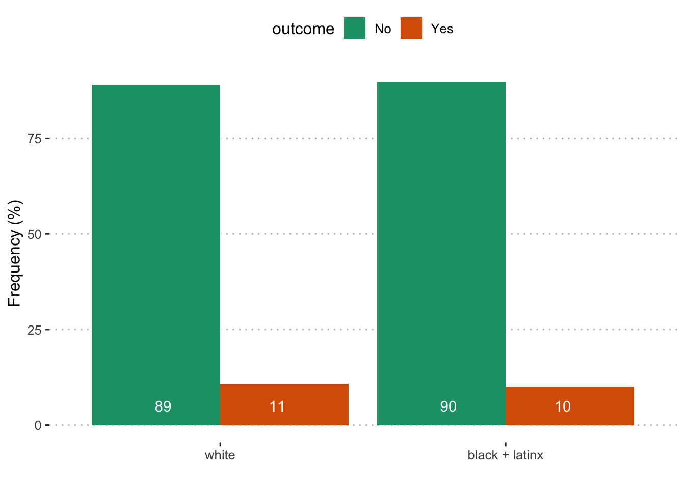
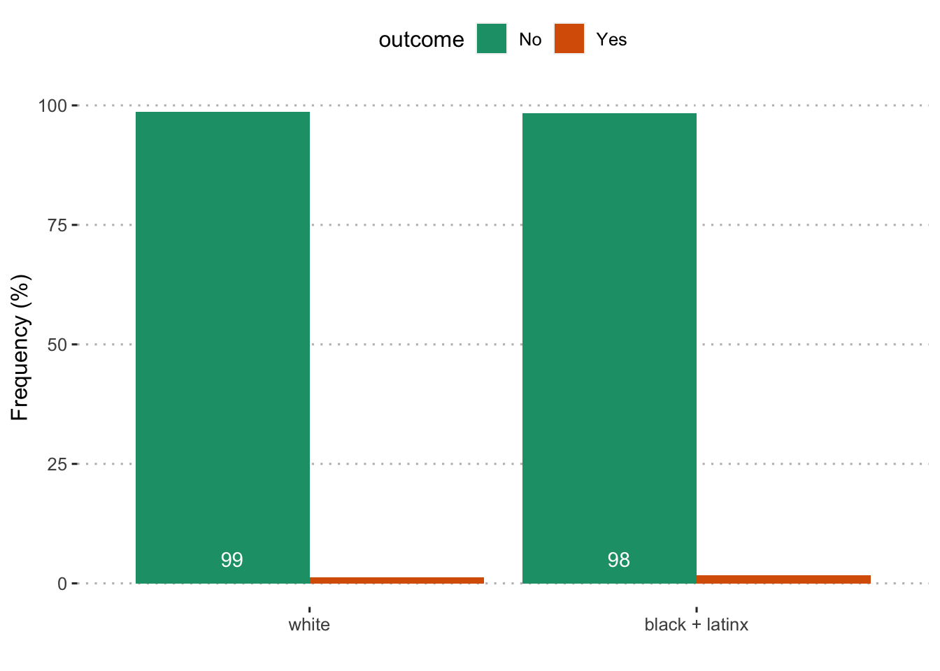
## X-squared = 1.4212, df = 1, p-value = 0.2332Black + LatinX
##
## Pearson's Chi-squared test with Yates' continuity correction
##
## data: scored$sick_leave and scored$compare2
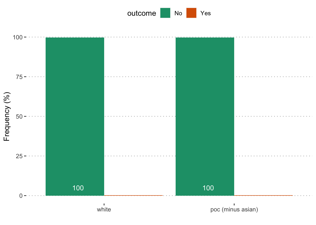
## X-squared = 0.27466, df = 1, p-value = 0.6002People of Color (minus Asian)
##
## Pearson's Chi-squared test with Yates' continuity correction
##
## data: scored$sick_leave and scored$compare3
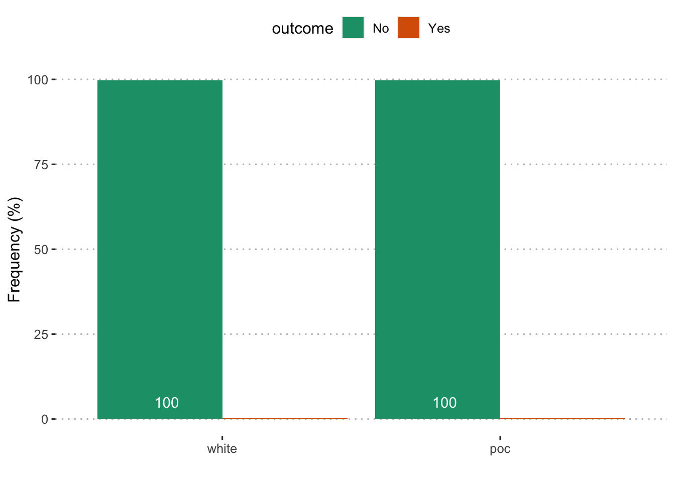
## X-squared = 0.00024085, df = 1, p-value = 0.9876People of Color
##
## Pearson's Chi-squared test with Yates' continuity correction
##
## data: scored$sick_leave and scored$compare4
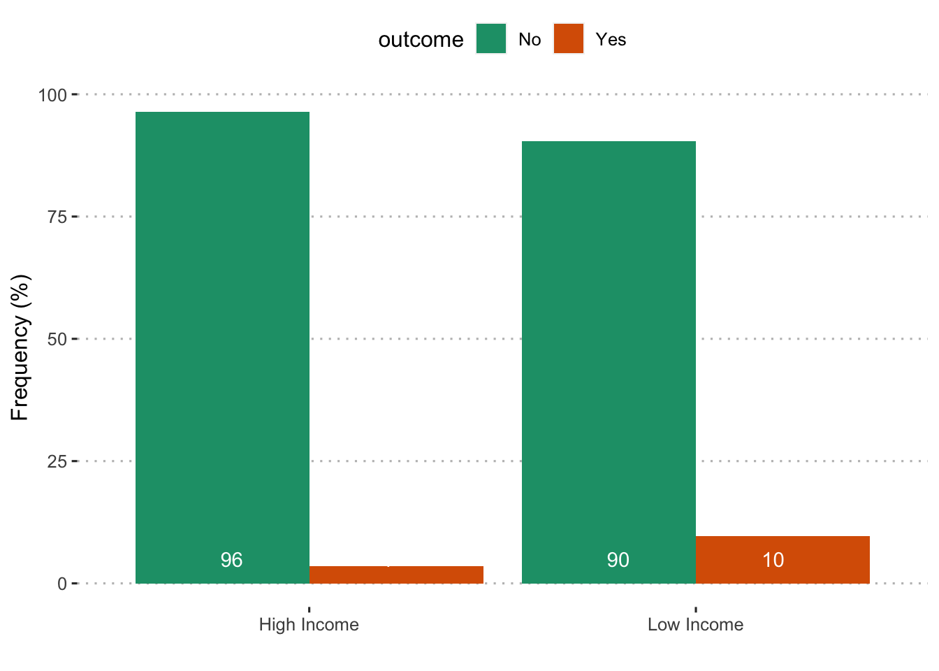
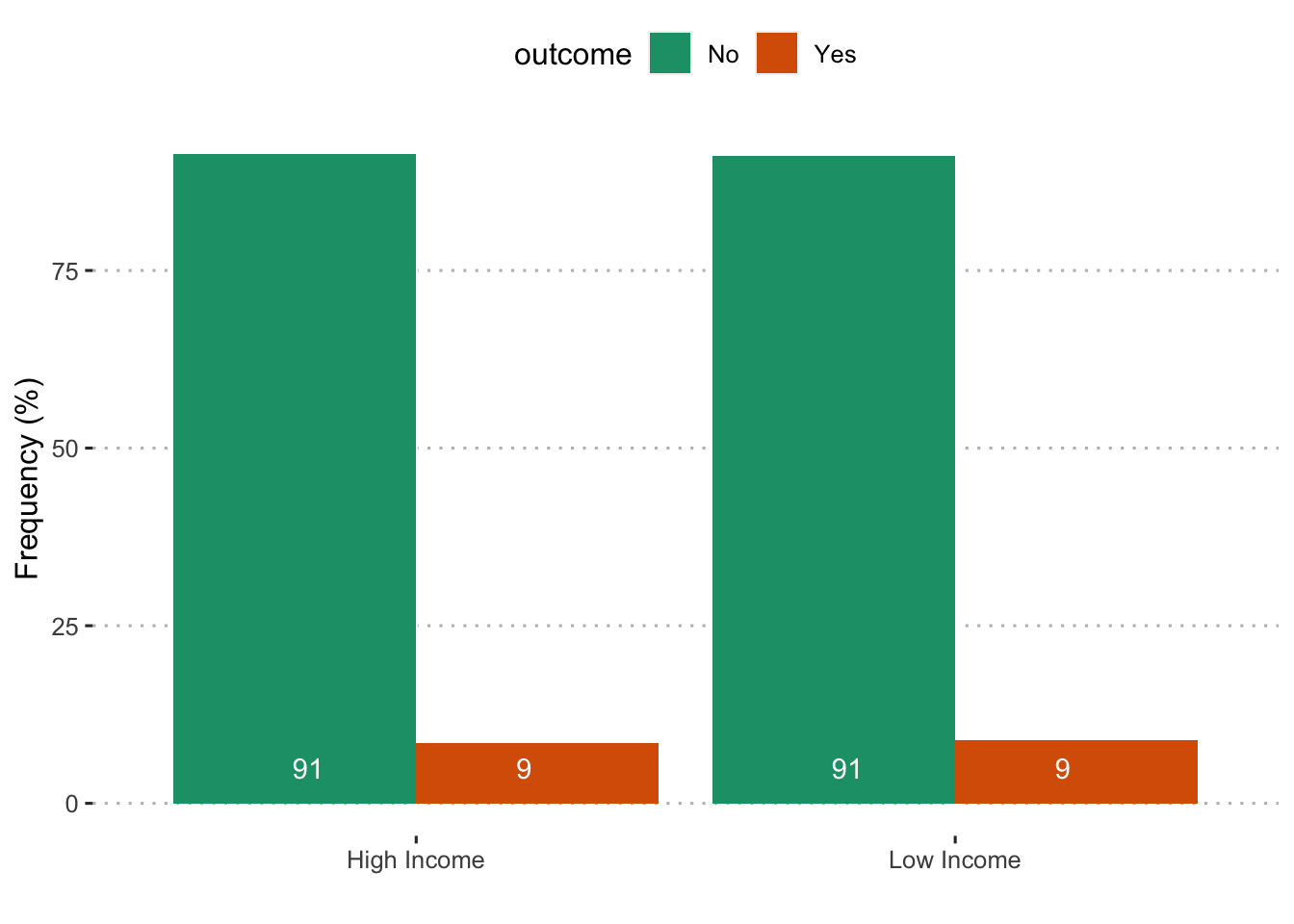
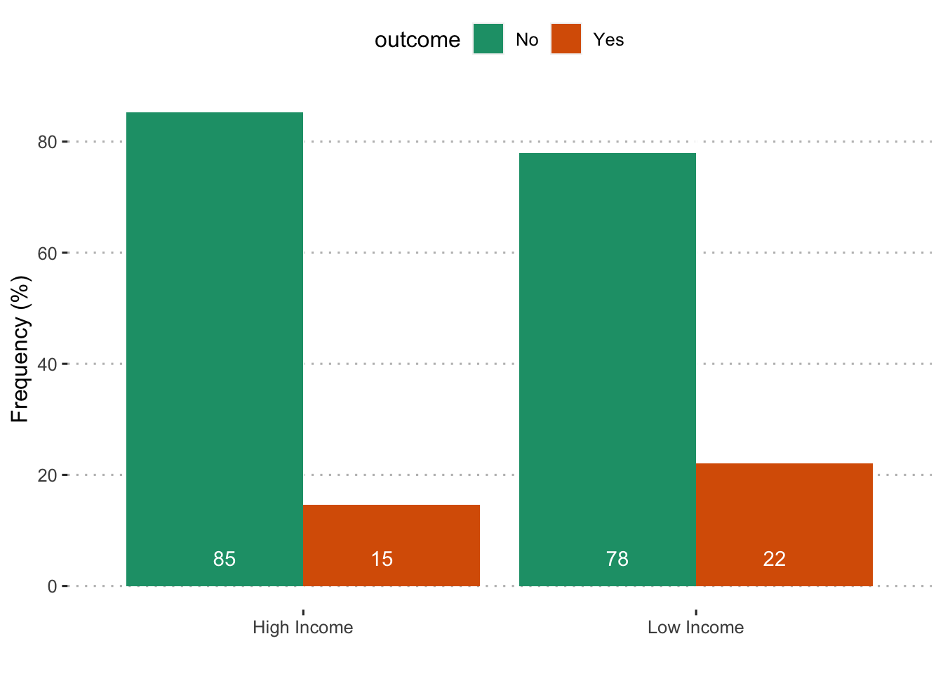
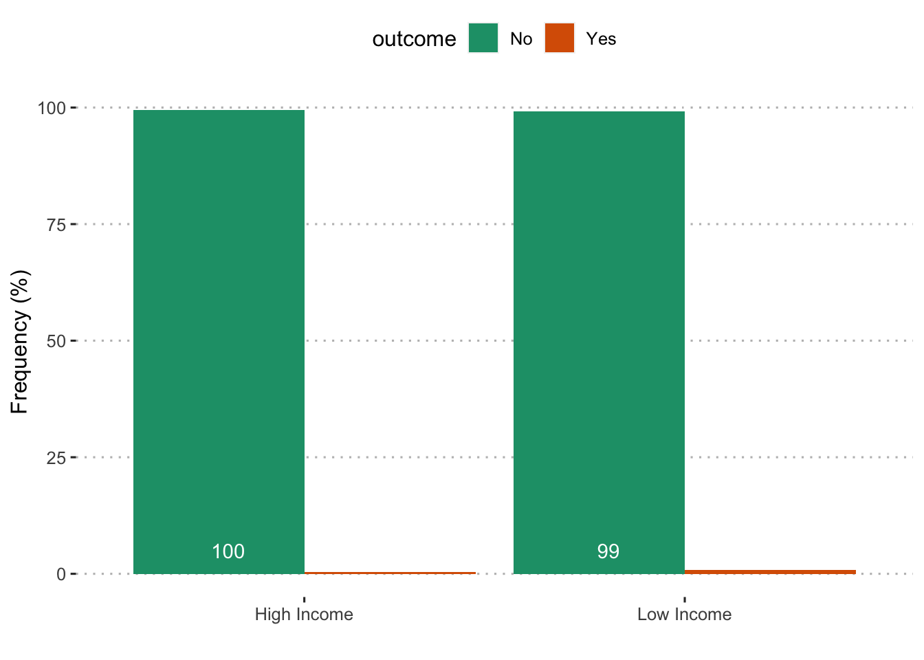
## X-squared = 0.074761, df = 1, p-value = 0.7845By income
##
## Pearson's Chi-squared test with Yates' continuity correction
##
## data: scored$sick_leave and scored$poverty150
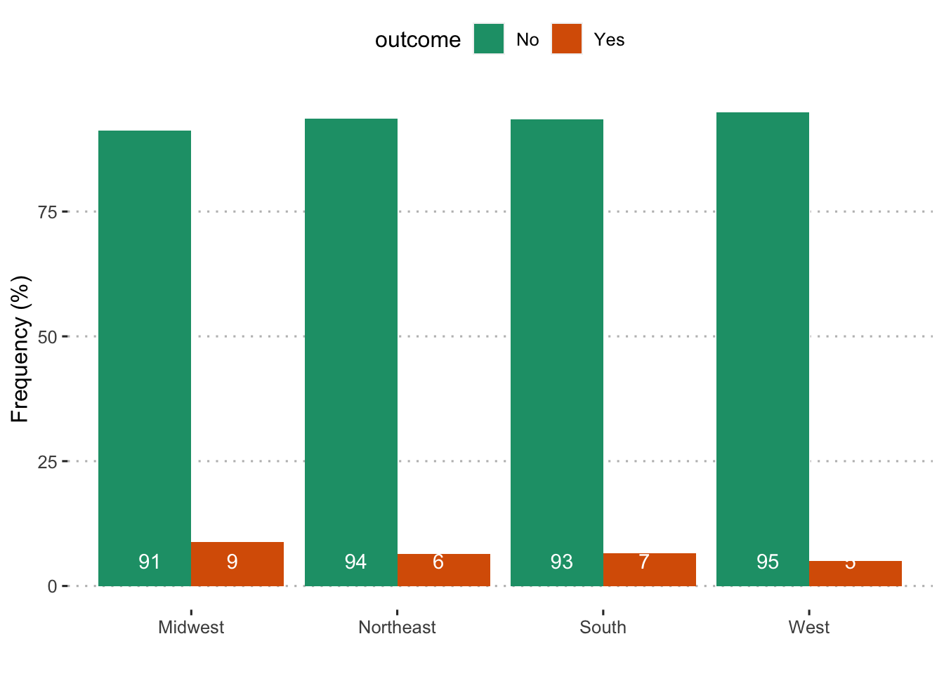
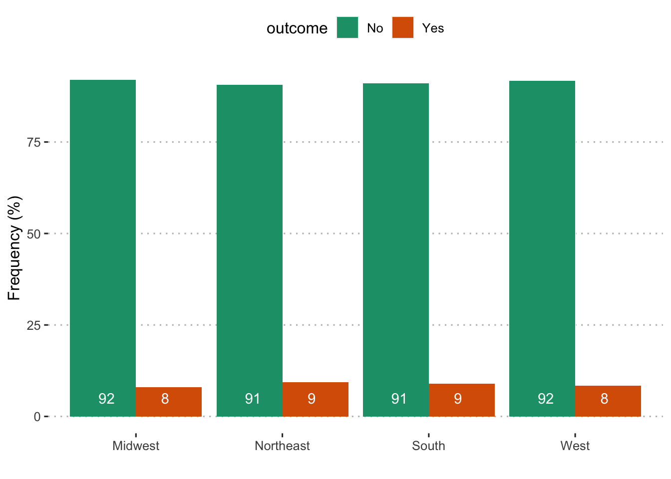
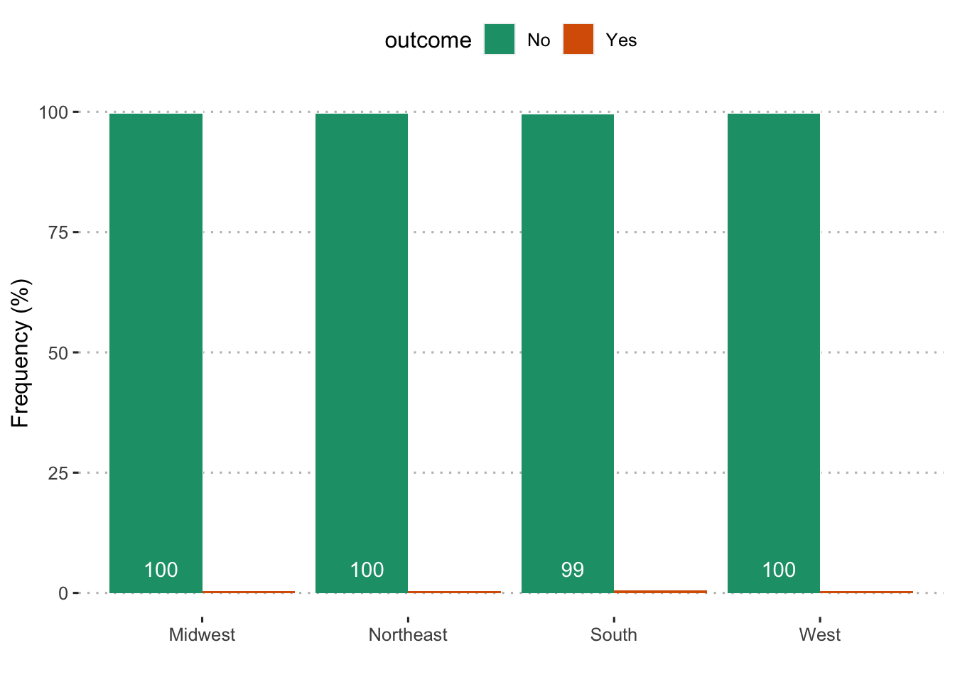
## X-squared = 407.09, df = 1, p-value < 2.2e-16Geographic Region
##
## Pearson's Chi-squared test
##
## data: scored$sick_leave and scored$region
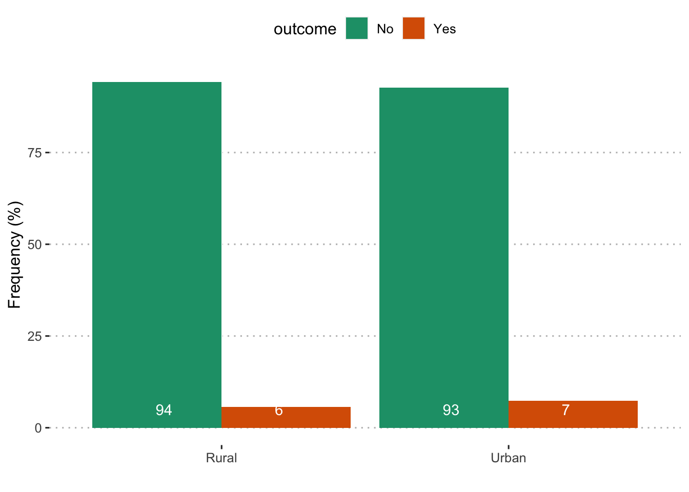
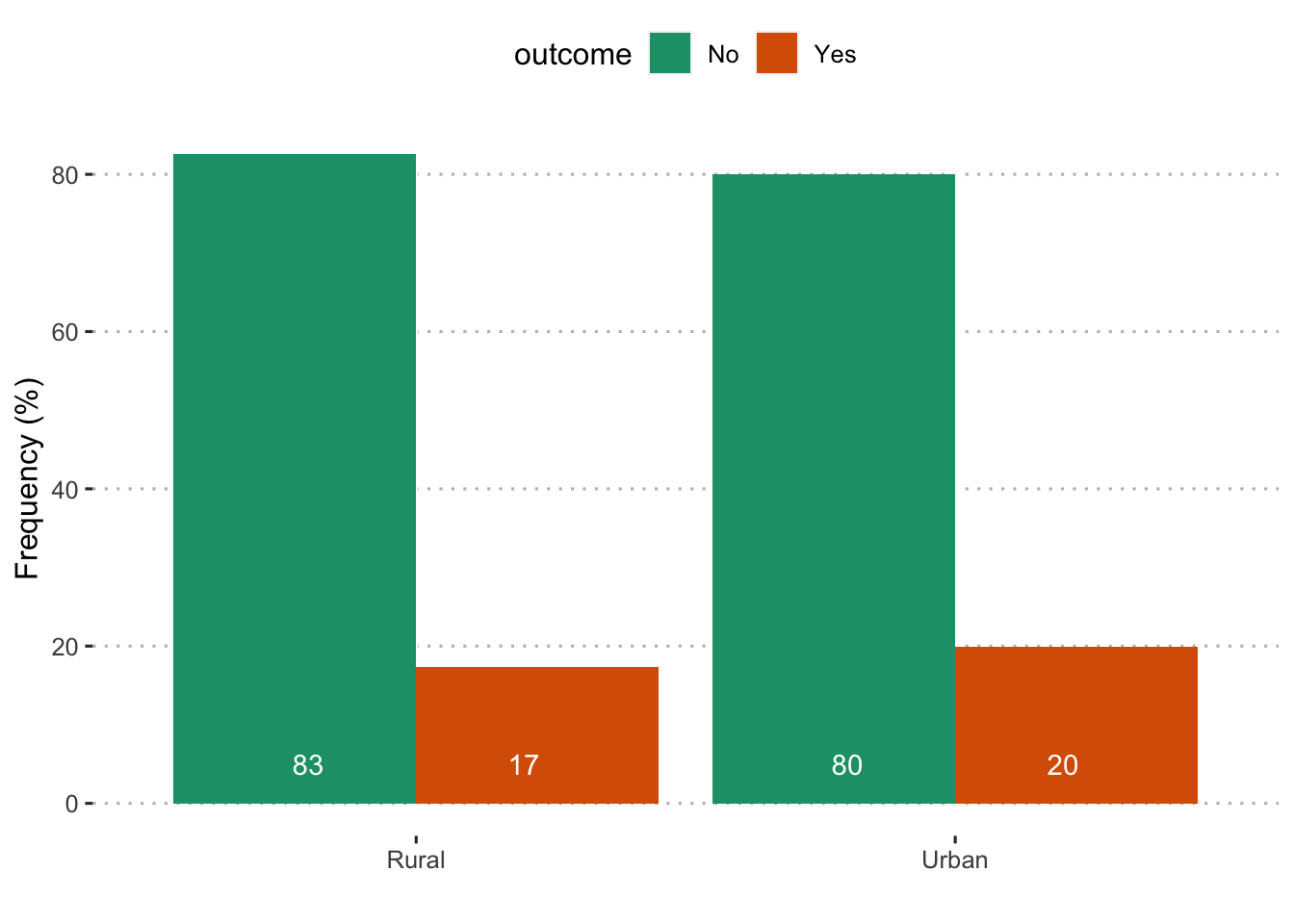
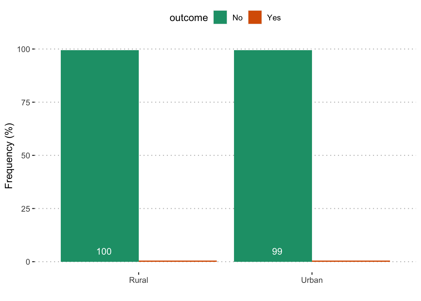
## X-squared = 58.52, df = 3, p-value = 1.217e-12Rural/Urban
##
## Pearson's Chi-squared test with Yates' continuity correction
##
## data: scored$sick_leave and scored$rural
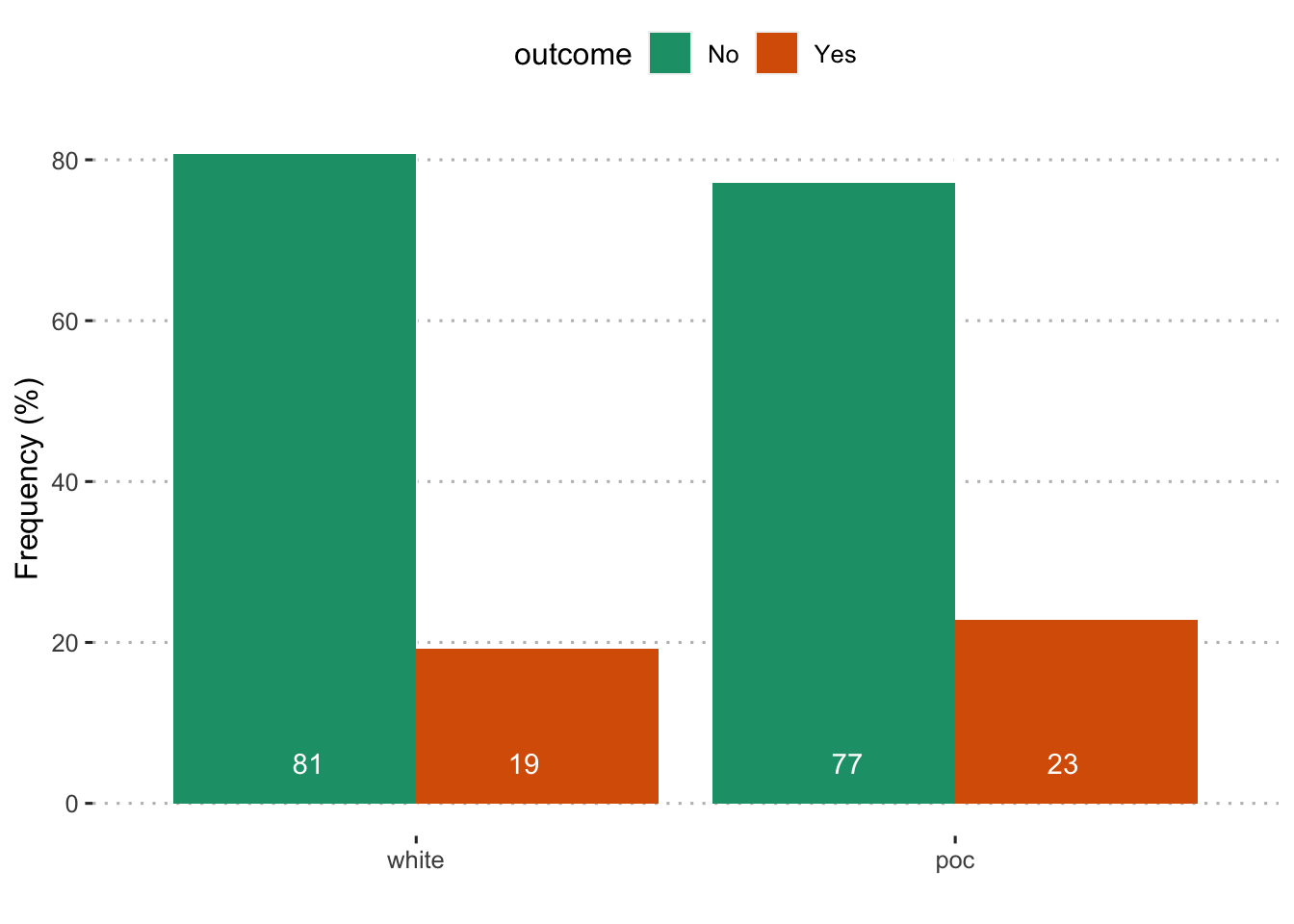
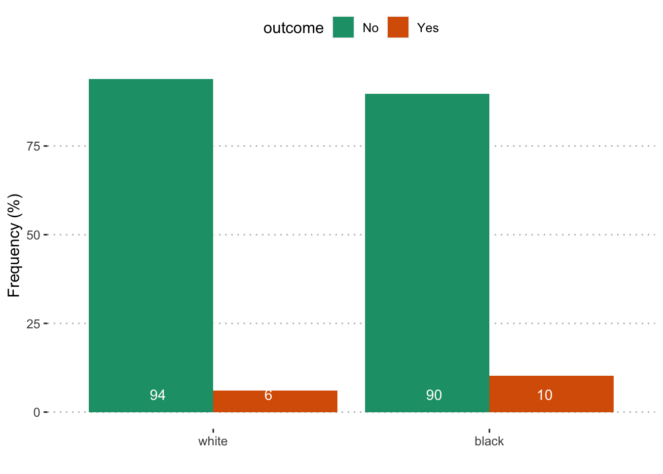
## X-squared = 21.556, df = 1, p-value = 3.436e-06Employment
Unemployed
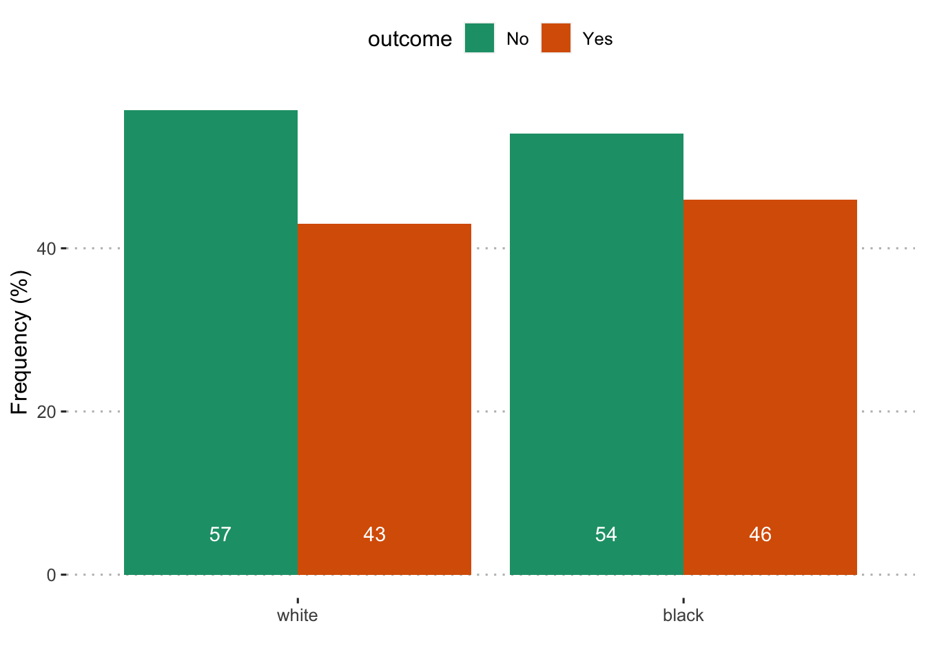
Black

##
## Pearson's Chi-squared test with Yates' continuity correction
##
## data: scored$unemployed and scored$compare1
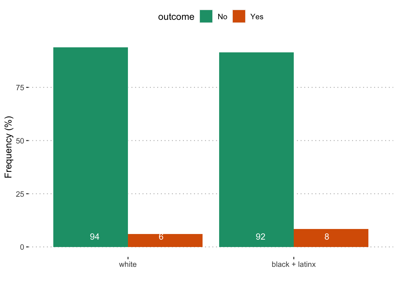
## X-squared = 4.8389, df = 1, p-value = 0.02783Black + LatinX

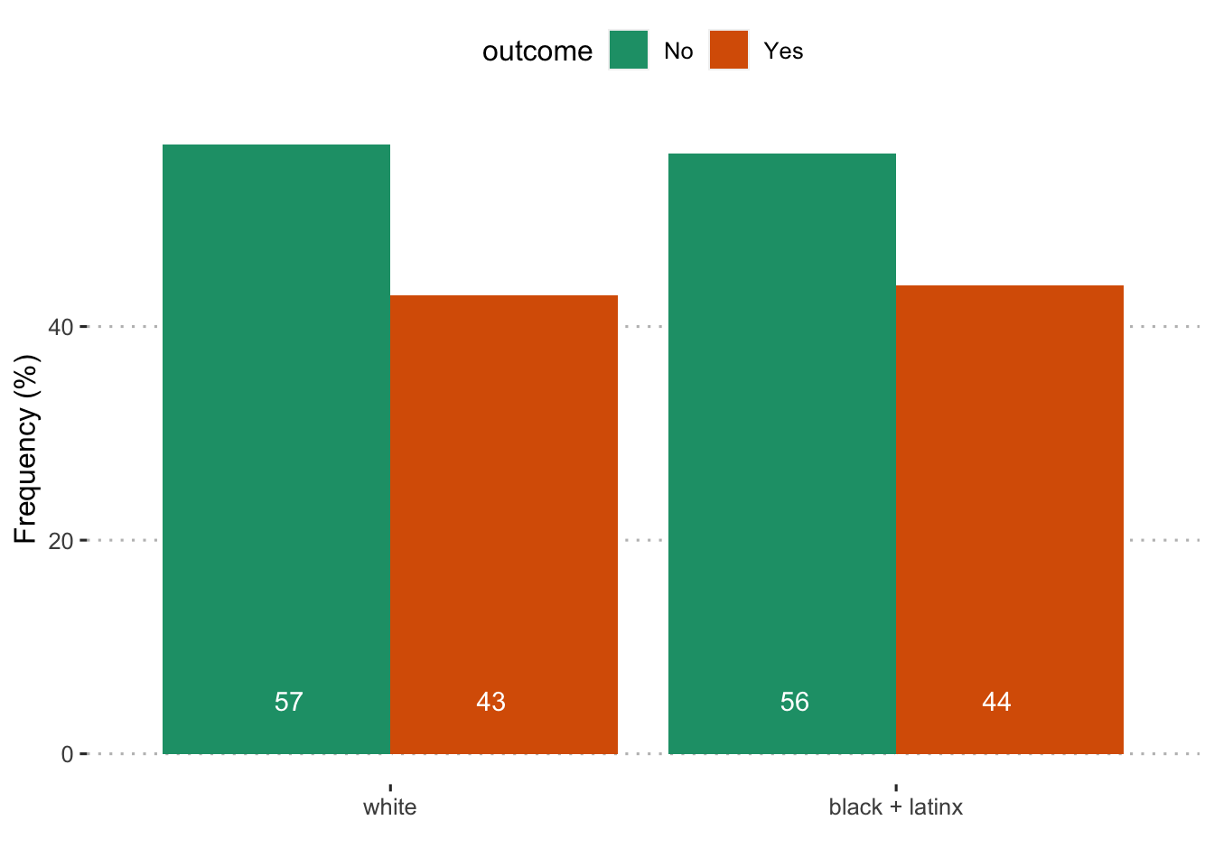
##
## Pearson's Chi-squared test with Yates' continuity correction
##
## data: scored$unemployed and scored$compare2
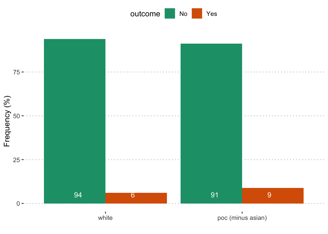
## X-squared = 15.485, df = 1, p-value = 8.315e-05People of Color (minus Asian)

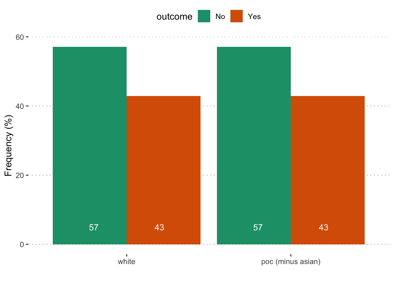
##
## Pearson's Chi-squared test with Yates' continuity correction
##
## data: scored$unemployed and scored$compare3
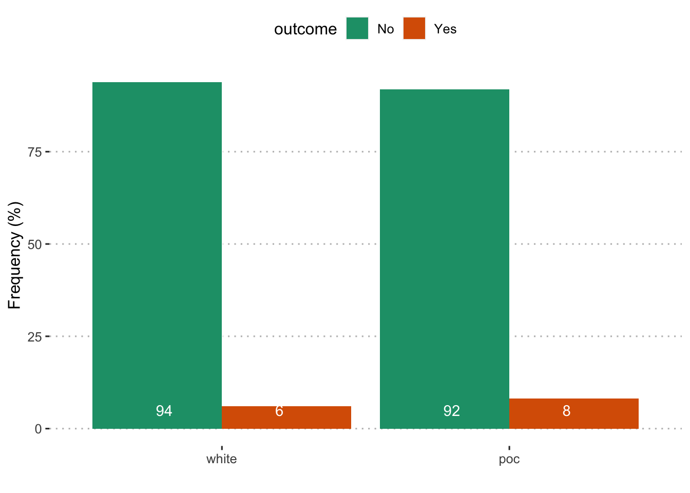
## X-squared = 17.15, df = 1, p-value = 3.453e-05People of Color
##
##  Pearson's Chi-squared test with Yates' continuity correction
##
## data:  scored$unemployed and scored$compare4
## X-squared = 14.95, df = 1, p-value = 0.0001104
By income
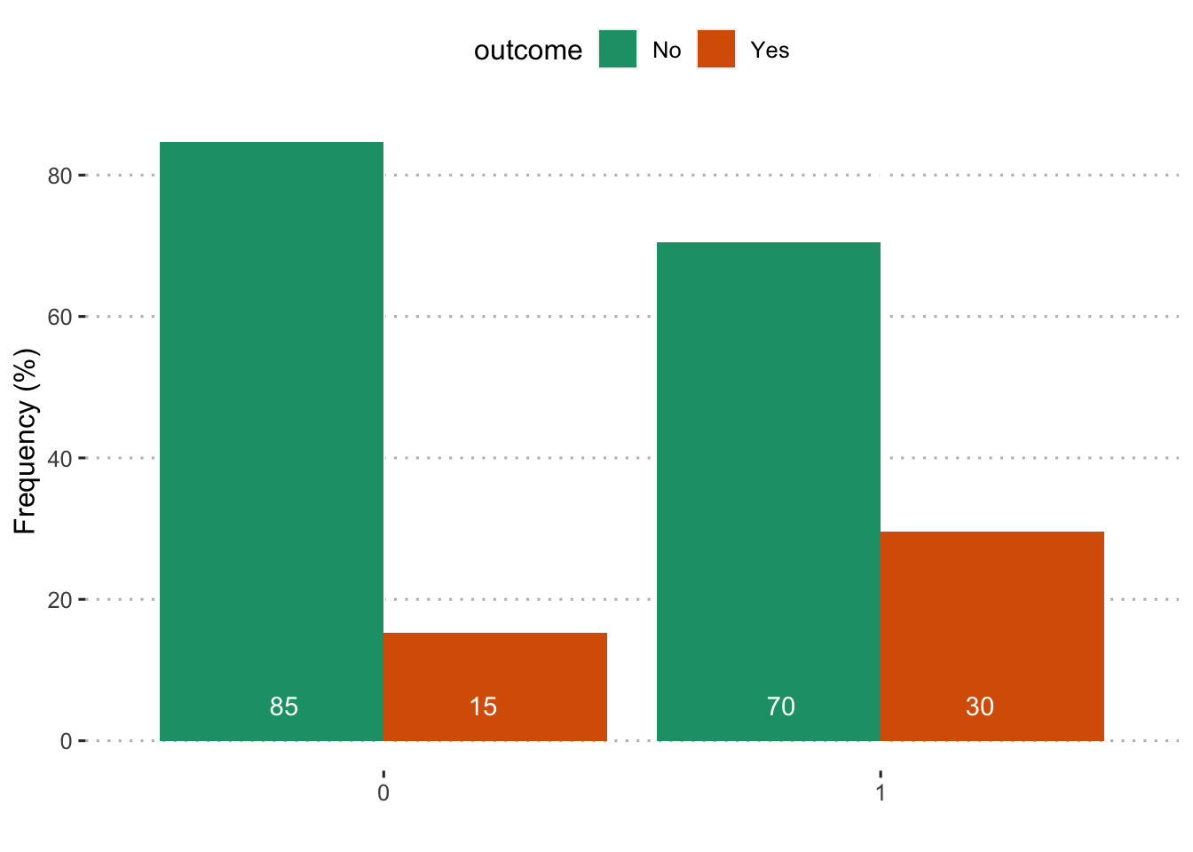
##
## Pearson's Chi-squared test with Yates' continuity correction
##
## data: scored$unemployed and scored$poverty150
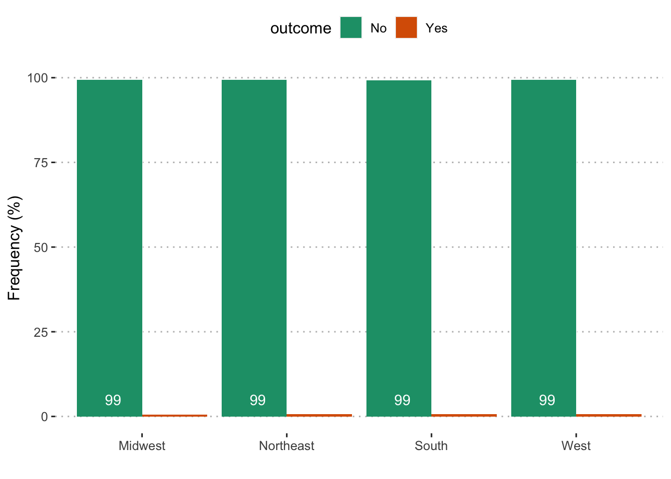
## X-squared = 219.93, df = 1, p-value < 2.2e-16Geographic Region
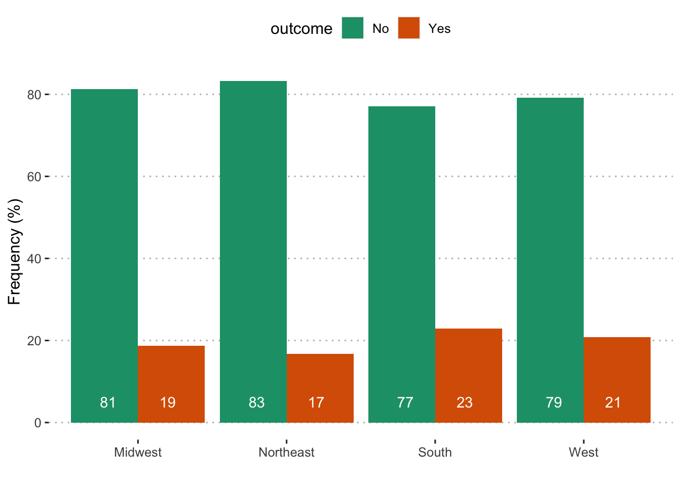
##
##  Pearson's Chi-squared test
##
## data:  scored$unemployed and scored$region
## X-squared = 27.241, df = 3, p-value = 5.241e-06
Rural/Urban
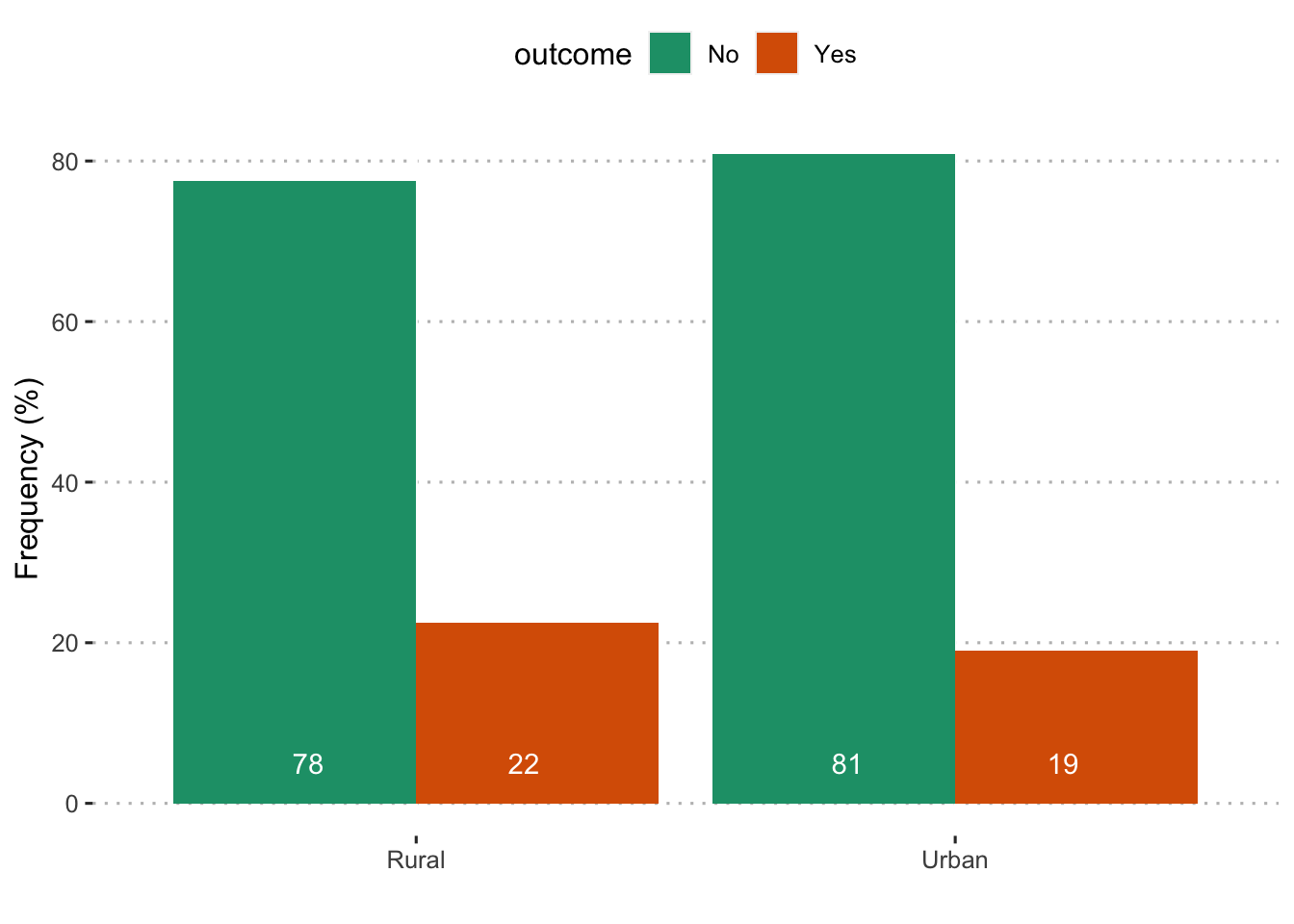
##
##  Pearson's Chi-squared test with Yates' continuity correction
##
## data:  scored$unemployed and scored$rural
## X-squared = 8.2554, df = 1, p-value = 0.004063
Lost employment
“Has your level of employment decreased due to the coronavirus (COVID-19) pandemic?”
Black
##
##  Pearson's Chi-squared test with Yates' continuity correction
##
## data:  scored$employment_decreased and scored$compare1
## X-squared = 27.033, df = 1, p-value = 2e-07
Black + LatinX

##
## Pearson's Chi-squared test with Yates' continuity correction
##
## data: scored$employment_decreased and scored$compare2
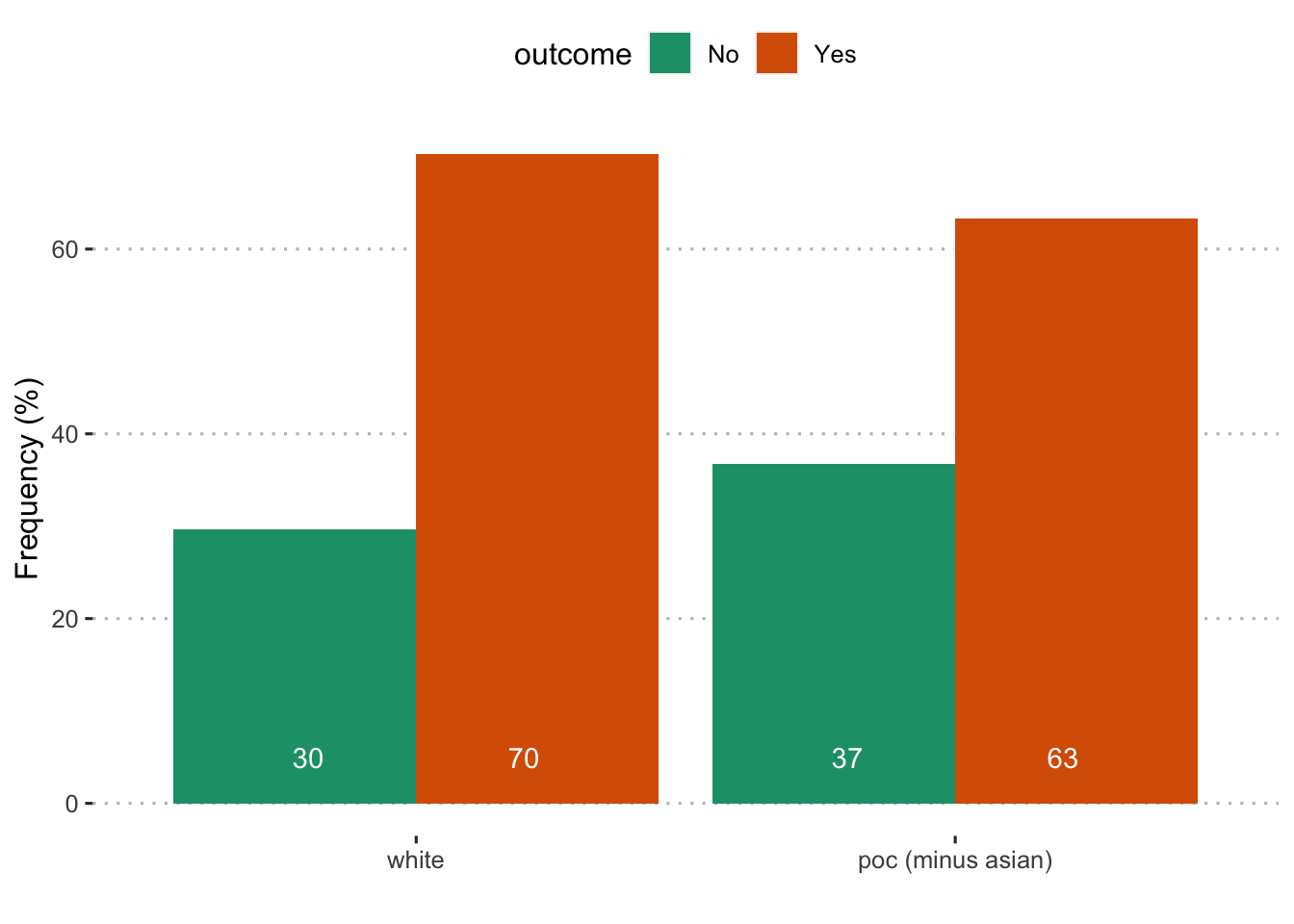
## X-squared = 74.038, df = 1, p-value < 2.2e-16People of Color (minus Asian)
##
## Pearson's Chi-squared test with Yates' continuity correction
##
## data: scored$employment_decreased and scored$compare3
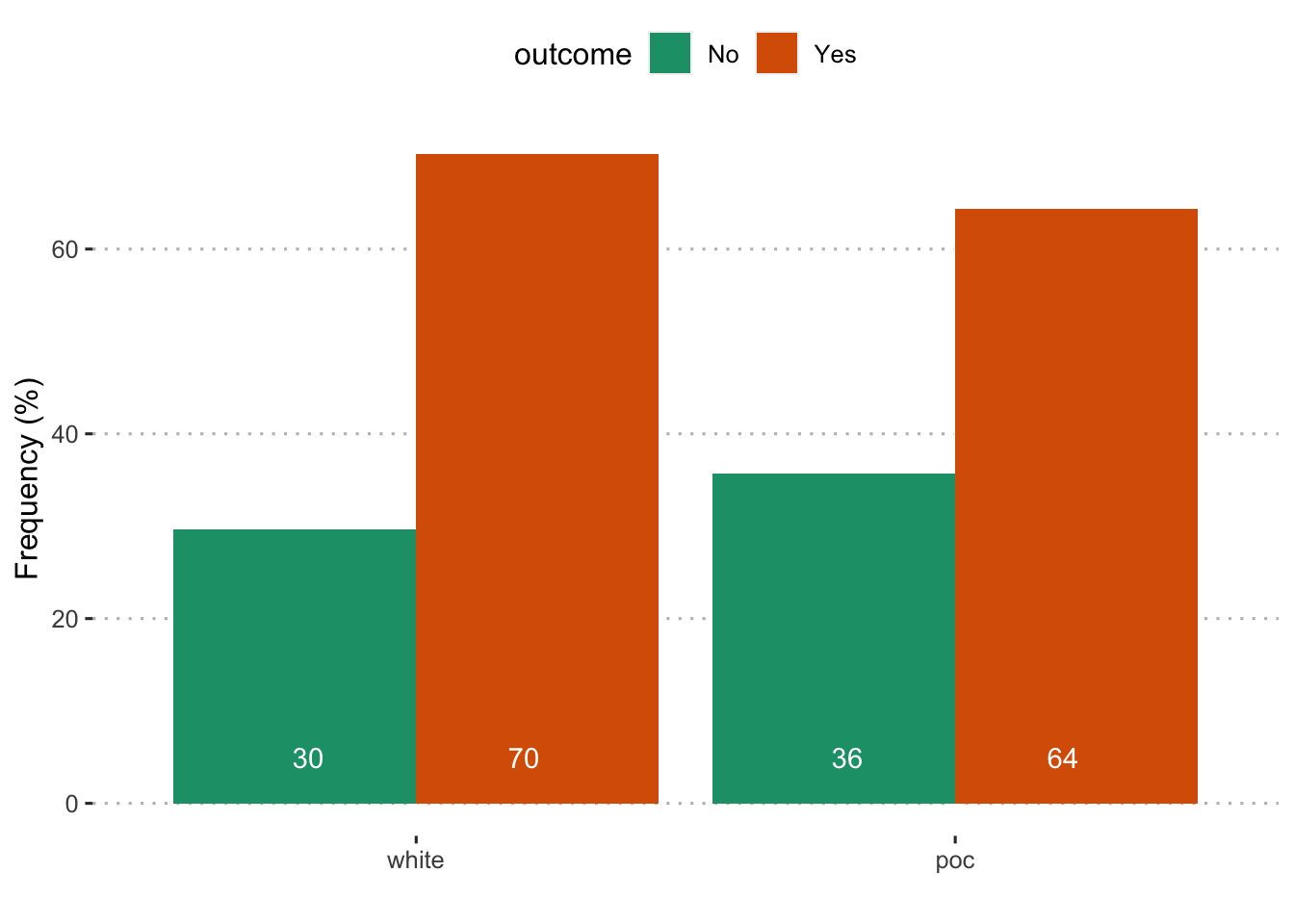
## X-squared = 81.018, df = 1, p-value < 2.2e-16People of Color
##
## Pearson's Chi-squared test with Yates' continuity correction
##
## data: scored$employment_decreased and scored$compare4
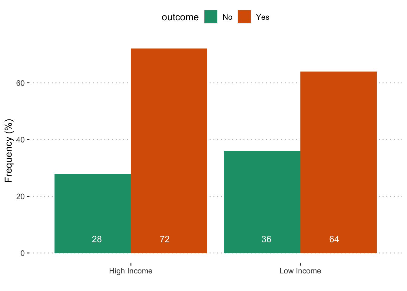
## X-squared = 72.955, df = 1, p-value < 2.2e-16By income
##
## Pearson's Chi-squared test with Yates' continuity correction
##
## data: scored$employment_decreased and scored$poverty150
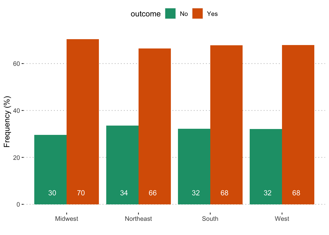
## X-squared = 181.22, df = 1, p-value < 2.2e-16Geographic Region
##
##  Pearson's Chi-squared test
##
## data:  scored$employment_decreased and scored$region
## X-squared = 1.9427, df = 3, p-value = 0.5844
Rural/Urban
##
##  Pearson's Chi-squared test with Yates' continuity correction
##
## data:  scored$employment_decreased and scored$rural
## X-squared = 2.5619, df = 1, p-value = 0.1095
Among unemployed
| Comparison | Group 1 | Group 2 |
|---|---|---|
| 1 | Black | White |
| 176 | 1272 | |
| 2 | Black + LatinX | White |
| 507 | 1113 | |
| 3 | POC (minus Asian) | White |
| 592 | 1113 | |
| 4 | POC | White |
| 654 | 1113 |
Have access to free food
Black
##
##  Pearson's Chi-squared test with Yates' continuity correction
##
## data:  unemployed$free_food and unemployed$compare1
## X-squared = 11.313, df = 1, p-value = 0.0007695
Black + LatinX
##
##  Pearson's Chi-squared test with Yates' continuity correction
##
## data:  unemployed$free_food and unemployed$compare2
## X-squared = 7.0257, df = 1, p-value = 0.008035
People of Color (minus Asian)
##
##  Pearson's Chi-squared test with Yates' continuity correction
##
## data:  unemployed$free_food and unemployed$compare3
## X-squared = 11.58, df = 1, p-value = 0.0006665
People of Color

##
##  Pearson's Chi-squared test with Yates' continuity correction
##
## data:  unemployed$free_food and unemployed$compare4
## X-squared = 5.3255, df = 1, p-value = 0.02102
By income
##
##  Pearson's Chi-squared test with Yates' continuity correction
##
## data:  unemployed$free_food and unemployed$poverty150
## X-squared = 244.22, df = 1, p-value < 2.2e-16
Geographic Region
##
##  Pearson's Chi-squared test
##
## data:  unemployed$free_food and unemployed$region
## X-squared = 4.7261, df = 3, p-value = 0.193
Rural/Urban
##
##  Pearson's Chi-squared test with Yates' continuity correction
##
## data:  unemployed$free_food and unemployed$rural
## X-squared = 0.30867, df = 1, p-value = 0.5785
Lost free lunch for child(ren)
Black
##
##  Pearson's Chi-squared test with Yates' continuity correction
##
## data:  unemployed$lost_free_lunch and unemployed$compare1
## X-squared = 3.7391, df = 1, p-value = 0.05315
Black + LatinX
##
##  Pearson's Chi-squared test with Yates' continuity correction
##
## data:  unemployed$lost_free_lunch and unemployed$compare2
## X-squared = 2.7094, df = 1, p-value = 0.09976
People of Color (minus Asian)
##
##  Pearson's Chi-squared test with Yates' continuity correction
##
## data:  unemployed$lost_free_lunch and unemployed$compare3
## X-squared = 3.825, df = 1, p-value = 0.05049
People of Color
##
##  Pearson's Chi-squared test with Yates' continuity correction
##
## data:  unemployed$lost_free_lunch and unemployed$compare4
## X-squared = 2.2655, df = 1, p-value = 0.1323
By income
##
##  Pearson's Chi-squared test with Yates' continuity correction
##
## data:  unemployed$lost_free_lunch and unemployed$poverty150
## X-squared = 23.075, df = 1, p-value = 1.558e-06
Geographic Region
##
##  Chi-squared test for given probabilities
##
## data:  unemployed$lost_free_lunch
## X-squared = 1686, df = 1806, p-value = 0.9789
Rural/Urban
##
##  Pearson's Chi-squared test with Yates' continuity correction
##
## data:  unemployed$lost_free_lunch and unemployed$rural
## X-squared = 0.85934, df = 1, p-value = 0.3539
Childcare
Plans for next month
Same as right now
Black
##
##  Pearson's Chi-squared test with Yates' continuity correction
##
## data:  scored$plan_cc_samenow and scored$compare1
## X-squared = 20.81, df = 1, p-value = 5.073e-06
Black + LatinX

##
##  Pearson's Chi-squared test with Yates' continuity correction
##
## data:  scored$plan_cc_samenow and scored$compare2
## X-squared = 22.375, df = 1, p-value = 2.243e-06
People of Color (minus Asian)
##
##  Pearson's Chi-squared test with Yates' continuity correction
##
## data:  scored$plan_cc_samenow and scored$compare3
## X-squared = 21.889, df = 1, p-value = 2.888e-06
People of Color
##
##  Pearson's Chi-squared test with Yates' continuity correction
##
## data:  scored$plan_cc_samenow and scored$compare4
## X-squared = 17.105, df = 1, p-value = 3.536e-05
By income
##
##  Pearson's Chi-squared test with Yates' continuity correction
##
## data:  scored$plan_cc_samenow and scored$poverty150
## X-squared = 28.128, df = 1, p-value = 1.136e-07
Geographic Region
##
##  Pearson's Chi-squared test
##
## data:  scored$plan_cc_samenow and scored$region
## X-squared = 3.7043, df = 3, p-value = 0.2952
Rural/Urban
##
##  Pearson's Chi-squared test with Yates' continuity correction
##
## data:  scored$plan_cc_samenow and scored$rural
## X-squared = 0.0015298, df = 1, p-value = 0.9688
Different arrangement
Black
##
##  Pearson's Chi-squared test with Yates' continuity correction
##
## data:  scored$plan_cc_differ and scored$compare1
## X-squared = 9.9784, df = 1, p-value = 0.001584
Black + LatinX
##
##  Pearson's Chi-squared test with Yates' continuity correction
##
## data:  scored$plan_cc_differ and scored$compare2
## X-squared = 10.671, df = 1, p-value = 0.001088
People of Color (minus Asian)

##
##  Pearson's Chi-squared test with Yates' continuity correction
##
## data:  scored$plan_cc_differ and scored$compare3
## X-squared = 7.5562, df = 1, p-value = 0.00598
People of Color
##
##  Pearson's Chi-squared test with Yates' continuity correction
##
## data:  scored$plan_cc_differ and scored$compare4
## X-squared = 6.1717, df = 1, p-value = 0.01298
By income
##
##  Pearson's Chi-squared test with Yates' continuity correction
##
## data:  scored$plan_cc_differ and scored$poverty150
## X-squared = 0.1158, df = 1, p-value = 0.7336
Geographic Region
##
##  Pearson's Chi-squared test
##
## data:  scored$plan_cc_differ and scored$region
## X-squared = 1.4694, df = 3, p-value = 0.6894
Rural/Urban

##
##  Pearson's Chi-squared test with Yates' continuity correction
##
## data:  scored$plan_cc_differ and scored$rural
## X-squared = 4.4619, df = 1, p-value = 0.03466
Same as during pandemic
Black
##
##  Pearson's Chi-squared test with Yates' continuity correction
##
## data:  scored$plan_cc_sameCOVID and scored$compare1
## X-squared = 0.67446, df = 1, p-value = 0.4115
Black + LatinX
##
##  Pearson's Chi-squared test with Yates' continuity correction
##
## data:  scored$plan_cc_sameCOVID and scored$compare2
## X-squared = 0.504, df = 1, p-value = 0.4777
People of Color (minus Asian)

##
##  Pearson's Chi-squared test with Yates' continuity correction
##
## data:  scored$plan_cc_sameCOVID and scored$compare3
## X-squared = 0.6699, df = 1, p-value = 0.4131
People of Color

##
##  Pearson's Chi-squared test with Yates' continuity correction
##
## data:  scored$plan_cc_sameCOVID and scored$compare4
## X-squared = 0.90868, df = 1, p-value = 0.3405
By income

##
##  Pearson's Chi-squared test with Yates' continuity correction
##
## data:  scored$plan_cc_sameCOVID and scored$poverty150
## X-squared = 0.086435, df = 1, p-value = 0.7688
Geographic Region
##
##  Pearson's Chi-squared test
##
## data:  scored$plan_cc_sameCOVID and scored$region
## X-squared = 3.0154, df = 3, p-value = 0.3893
Rural/Urban
##
##  Pearson's Chi-squared test with Yates' continuity correction
##
## data:  scored$plan_cc_sameCOVID and scored$rural
## X-squared = 4.5959, df = 1, p-value = 0.03205
Don’t know
Black
##
##  Pearson's Chi-squared test with Yates' continuity correction
##
## data:  scored$plan_cc_dontknow and scored$compare1
## X-squared = 14.216, df = 1, p-value = 0.000163
Black + LatinX

##
##  Pearson's Chi-squared test with Yates' continuity correction
##
## data:  scored$plan_cc_dontknow and scored$compare2
## X-squared = 13.412, df = 1, p-value = 0.00025
People of Color (minus Asian)
##
##  Pearson's Chi-squared test with Yates' continuity correction
##
## data:  scored$plan_cc_dontknow and scored$compare3
## X-squared = 16.14, df = 1, p-value = 5.883e-05
People of Color

##
##  Pearson's Chi-squared test with Yates' continuity correction
##
## data:  scored$plan_cc_dontknow and scored$compare4
## X-squared = 14.656, df = 1, p-value = 0.000129
By income
##
##  Pearson's Chi-squared test with Yates' continuity correction
##
## data:  scored$plan_cc_dontknow and scored$poverty150
## X-squared = 33.766, df = 1, p-value = 6.214e-09
Geographic Region

##
##  Pearson's Chi-squared test with Yates' continuity correction
##
## data:  scored$plan_cc_dontknow and scored$poverty150
## X-squared = 33.766, df = 1, p-value = 6.214e-09
Rural/Urban
##
##  Pearson's Chi-squared test with Yates' continuity correction
##
## data:  scored$plan_cc_dontknow and scored$rural
## X-squared = 2.7611, df = 1, p-value = 0.09658
Lost type of childcare
Black
##
##  Pearson's Chi-squared test with Yates' continuity correction
##
## data:  scored$lostCC and scored$compare1
## X-squared = 0.40809, df = 1, p-value = 0.5229
Black + LatinX
##
##  Pearson's Chi-squared test with Yates' continuity correction
##
## data:  scored$lostCC and scored$compare2
## X-squared = 1.7122, df = 1, p-value = 0.1907
People of Color (minus Asian)
##
##  Pearson's Chi-squared test with Yates' continuity correction
##
## data:  scored$lostCC and scored$compare3
## X-squared = 1.1796, df = 1, p-value = 0.2774
People of Color

##
##  Pearson's Chi-squared test with Yates' continuity correction
##
## data:  scored$lostCC and scored$compare4
## X-squared = 0.74367, df = 1, p-value = 0.3885
By income

##
##  Pearson's Chi-squared test with Yates' continuity correction
##
## data:  scored$plan_cc_dontknow and scored$poverty150
## X-squared = 33.766, df = 1, p-value = 6.214e-09
Geographic Region
##
##  Pearson's Chi-squared test
##
## data:  scored$plan_cc_dontknow and scored$region
## X-squared = 1.1743, df = 3, p-value = 0.7592
Rural/Urban
##
##  Pearson's Chi-squared test with Yates' continuity correction
##
## data:  scored$lostCC and scored$rural
## X-squared = 0.56361, df = 1, p-value = 0.4528
Type of care for the next month
Center-based
Black

##
##  Pearson's Chi-squared test with Yates' continuity correction
##
## data:  scored$expect_center and scored$compare1
## X-squared = 0.73597, df = 1, p-value = 0.391
Black + LatinX
##
##  Pearson's Chi-squared test with Yates' continuity correction
##
## data:  scored$expect_center and scored$compare2
## X-squared = 2.6121, df = 1, p-value = 0.106
People of Color (minus Asian)

##
##  Pearson's Chi-squared test with Yates' continuity correction
##
## data:  scored$expect_center and scored$compare3
## X-squared = 1.2627, df = 1, p-value = 0.2611
People of Color

##
##  Pearson's Chi-squared test with Yates' continuity correction
##
## data:  scored$expect_center and scored$compare4
## X-squared = 0.93472, df = 1, p-value = 0.3336
By income

##
##  Pearson's Chi-squared test with Yates' continuity correction
##
## data:  scored$expect_center and scored$poverty150
## X-squared = 1.6588, df = 1, p-value = 0.1978
Geographic Region
##
##  Pearson's Chi-squared test
##
## data:  scored$expect_center and scored$region
## X-squared = 2.4723, df = 3, p-value = 0.4803
Rural/Urban
##
##  Pearson's Chi-squared test with Yates' continuity correction
##
## data:  scored$expect_center and scored$rural
## X-squared = 0.013, df = 1, p-value = 0.9092
Care by relatives
Black

##
##  Pearson's Chi-squared test with Yates' continuity correction
##
## data:  scored$expect_relative and scored$compare1
## X-squared = 0.028474, df = 1, p-value = 0.866
Black + LatinX

##
##  Pearson's Chi-squared test with Yates' continuity correction
##
## data:  scored$expect_relative and scored$compare2
## X-squared = 2.3755, df = 1, p-value = 0.1233
People of Color (minus Asian)

##
##  Pearson's Chi-squared test with Yates' continuity correction
##
## data:  scored$expect_relative and scored$compare3
## X-squared = 2.4451, df = 1, p-value = 0.1179
People of Color

##
##  Pearson's Chi-squared test with Yates' continuity correction
##
## data:  scored$expect_relative and scored$compare4
## X-squared = 1.6884, df = 1, p-value = 0.1938
By income
##
##  Pearson's Chi-squared test with Yates' continuity correction
##
## data:  scored$expect_relative and scored$poverty150
## X-squared = 3.1149, df = 1, p-value = 0.07758
Geographic Region
##
##  Pearson's Chi-squared test
##
## data:  scored$expect_relative and scored$region
## X-squared = 0.51307, df = 3, p-value = 0.916
Rural/Urban
##
##  Pearson's Chi-squared test with Yates' continuity correction
##
## data:  scored$expect_relative and scored$rural
## X-squared = 0.005328, df = 1, p-value = 0.9418
Professional (non-centerbased)
Black
##
##  Pearson's Chi-squared test with Yates' continuity correction
##
## data:  scored$expect_pro and scored$compare1
## X-squared = 3.448e-27, df = 1, p-value = 1
Black + LatinX

##
##  Pearson's Chi-squared test with Yates' continuity correction
##
## data:  scored$expect_pro and scored$compare2
## X-squared = 0.091306, df = 1, p-value = 0.7625
People of Color (minus Asian)
##
##  Pearson's Chi-squared test with Yates' continuity correction
##
## data:  scored$expect_pro and scored$compare3
## X-squared = 2.0345e-26, df = 1, p-value = 1
People of Color
##
##  Pearson's Chi-squared test with Yates' continuity correction
##
## data:  scored$expect_pro and scored$compare4
## X-squared = 2.7225e-27, df = 1, p-value = 1
By income

##
##  Pearson's Chi-squared test with Yates' continuity correction
##
## data:  scored$expect_pro and scored$poverty150
## X-squared = 6.1753e-27, df = 1, p-value = 1
Geographic Region
##
##  Pearson's Chi-squared test
##
## data:  scored$expect_pro and scored$region
## X-squared = 3.631, df = 3, p-value = 0.3042
Rural/Urban

##
##  Pearson's Chi-squared test with Yates' continuity correction
##
## data:  scored$expect_pro and scored$rural
## X-squared = 0.029907, df = 1, p-value = 0.8627